Proof.
The proof consists of three main steps. In order to diagonalize
Hamiltonian (
4), we
- apply the Lemma to simplify the Hamiltonian using the peakness
of the kernels,
- perform Bogolyubov transformation to diagonalize the
 part
of the Hamiltonian,
part
of the Hamiltonian,
- make a near-identity canonical transformation to diagonalize the
 part of the Hamiltonian.
Step 1: Applying Lemma.
Similarly to Eq. (
26), we can write a filtered Hamiltonian
for Eq. (
4) as
here, as usual c.c. stands for complex conjugate. From
property (
65) and definition (
68) it follows
that
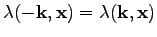
.
Step 2: Bogolyubov transformation.
In this step we apply the usual Bogolyubov transformation.
Before
doing that notice that Hamiltonian (
71) consists of two
parts
where
are correspondingly
and
parts of

. In Step
2, we diagonalize the
part using the following linear
transformation
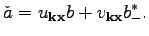 |
|
|
(66) |
It was shown in [
10] that transformation (
73)
is canonical if the following conditions are satisfied:
Let us follow [
10] and choose
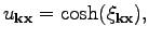 |
|
|
(67) |
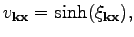 |
|
|
(68) |
where

is real and even, but otherwise arbitrary function.
Then under change of variables given by Eq. (
73),

becomes
Denote an expression in square brackets multiplying

as

:
Using trigonometric formulas for hyperbolic functions, we obtain
 |
|
|
(69) |
In order to diagonalize
, we require that the
following condition in satisfied
 |
|
|
(70) |
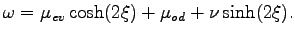
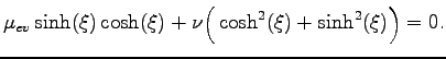
This condition is equivalent to
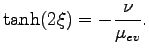 |
|
|
(71) |
Since

, we can choose

to be positive and,
therefore, we have
In Appendix
B, we find the expression for

.
Resolving Eq. (
76) together with Eqs. (
79) and (
80), we obtain
Therefore, we have diagonalized
to the form
 |
|
|
(74) |
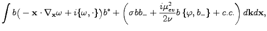
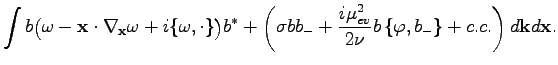
Next, we consider the
part of the filtered
Hamiltonian. In Appendix
C, we show that
Bogolyubov transformation (
73) transforms

to the form
where
Combining Eqs. (
81) and (
82), we
finally obtain Hamiltonian in the form
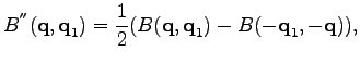
Step 3: Near-identity transformation.
In Step 2, we diagonalized
part but not all of the
part. In order to diagonalize complete Hamiltonian,
we use the near-identity transformation. This near-identity
transformation changes variables from

to

by the
following rule
 |
|
|
(76) |
where, we assume that

and

are
terms and

and
are
which makes our
transformation indeed near identical. Note that
,
, and
are functions of both

and

. Nevertheless, for
simplicity of notation, we do omit the dependence on
, since it
would only unnecessarily pollute the notations. In
Appendix
D, we derive the canonicity conditions for
transformation (
84). In turns out that
transformation (
84) is canonical if the following conditions
are met
Among the coefficients
,
and
that satisfy the
canonicity conditions we have to choose those that will diagonalize
the
part. In Appendix
E, we show that
such coefficients become
Note that these conditions are
in full correspondence with the canonicity conditions (
85).
The Hamiltonian in new variables up to
order is
This completes the proof of the main result of this paper.


![$\displaystyle \int \Big[\mu\cosh^2(\xi)+\mu_-\sinh^2(\xi)+2\nu\sinh(\xi)\cosh(\xi)\Big]
\vert b\vert^2d\textbf{k}d\textbf{x}$](img290.png)
d\textbf{k}d\textbf{x}$](img291.png)
![$\displaystyle \omega = \Big[\mu\cosh^2(\xi)+\mu_-\sinh^2(\xi)+
2\nu\sinh(\xi)\cosh(\xi)\Big].
$](img294.png)

![$\displaystyle H_f=\int c[\omega -\textbf{x}\cdot\nabla_\textbf{x}\omega +i\{\omega ,\cdot\}]c^*d\textbf{k}d\textbf{x}$](img334.png)

![$\displaystyle H_f=\int c_{\textbf{k}\textbf{x}}[\omega -\textbf{x}\cdot\nabla_\...
...x}\omega +i\{\omega ,\cdot\}]
c_{\textbf{k}\textbf{x}}^*d\textbf{k}d\textbf{x}.$](img270.png)
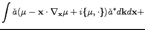
![$\displaystyle \frac{1}{2}\int [\check{a}[\lambda-\textbf{x}\cdot\nabla_{\textbf{x}}\lambda+i\{\lambda,\cdot\}]\check{a}_{-}d\textbf{k}d\textbf{x}+c.c.],$](img275.png)
![$\displaystyle \int\mu \vert\check{a}\vert^2d\textbf{k}d\textbf{x}+\frac{1}{2}
\int \nu [\check{a}\check{a}_-+\check{a}^*\check{a}_-^*]d\textbf{k}d\textbf{x},$](img279.png)