Proof.
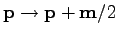
In order to obtain the new variables

, we first make a
window transform via (
17), which is then followed by a
near-identical transformation to the new variables
. The
idea of the proof is to use the peakness of the kernel

. We make a Taylor expansion around the peak and
then by neglecting the higher order terms we obtain the desired
result.
We make a window transform from
 to
to
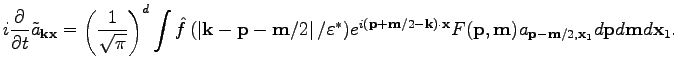
 using Eq. (20).
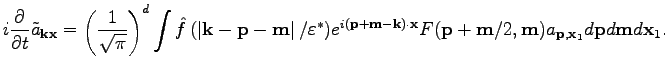
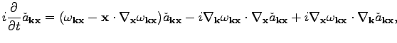
Differentiating Eq. (20) with respect to time, using the Eq. (25), and applying the inverse
formula (21) yield
using Eq. (20).
Differentiating Eq. (20) with respect to time, using the Eq. (25), and applying the inverse
formula (21) yield
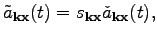
Let us change variables from

to

as
Below it will be convenient to use
 |
|
|
(29) |
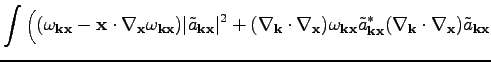
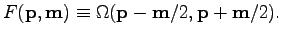
Next, we will approximate the RHS of Eq. (
28) by a
variation of some filtered Hamiltonian

, i.e., by

. We can rewrite Eq. (
28) as
 |
|
|
(30) |
Let us make another change of variables
 |
|
|
(31) |
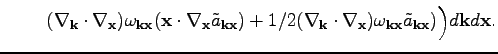
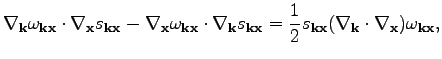
In order to simplify Eq. (
33), we are going to use the fact
that

and

are peaked functions of

and

, respectively, and fast decaying at infinity. We also keep
only first order terms in spatial derivatives, neglecting second and
higher order terms. Then, we could write
 h.o.t. h.o.t. |
|
|
(32) |
Similarly, we obtain
 h.o.t. h.o.t. |
|
|
(33) |
where h.o.t. denotes higher order terms. Now, we substitute the
expansions (
34) and (
35) into
Eq. (
32), and after ignoring higher order terms, we obtain
Note that, here we have an expansion with two different small
parameters

and

, which obey Eq. (
18).
In Appendix A, we show how to simplify the RHS of
Eq. (36). As a result of this simplification, we obtain
This equation can be written in the Hamiltonian form
where the filtered Hamiltonian takes form
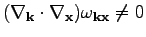
Now, we will use the general method of the WKB approximation. We will
only keep the terms, which are of the first order in a small parameter
.
In our case, the small parameter
characterizes the rate of
spatial change of the position dependent frequency

and the
dynamical variable
. To apply the WKB approximation to
Eq. (
37), we neglect the terms that have two derivatives
with respect to

(underlined) because each spatial derivative is of the order
small. As a result, we obtain the
following equation of motion
 |
|
|
(36) |
However, Eq. (
39) becomes non-Hamiltonian. Indeed, the
corresponding functional
 |
|
|
|
 |
|
|
(37) |
is not self-conjugate if
. Therefore, in order
to obtain canonical equations of motion, another near-canonical change
of variables needs to be performed
 |
|
|
(38) |
where

is some time-independent function to be determined
below. Note that transformation (
41) is canonical if
and only if
Therefore, we need to find such
that the system becomes
Hamiltonian in terms of new variables
and the
transformation (
41) is near-canonical, i.e.,

. We substitute Eq. (
41) into
Eq. (
39) to obtain
If we find
that satisfies the equation
 |
|
|
(39) |
then the equation of motion in the new variables
takes
the canonical form
 |
|
|
(40) |
with the corresponding Hamiltonian (
26). In order to find
a solution of Eq. (
42), we make a change of variables
 |
|
|
(41) |
to obtain
 |
|
|
(42) |
We find the solution of Eq. (
45) using the method of
characteristics. The characteristics

are given
by the following equations
where

is a parameter along the characteristics. Physically these characteristics
correspond to the trajectories (rays) of WKB wavepackets in the

space.
The solution of Eq. (
45) is given by
Now, we use Eq. (
44) and then Eq. (
41) in order
to obtain the new variable
out of the Gabor variable
. The dynamics of the new variable
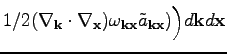
is
described by the filtered Hamiltonian (
26).


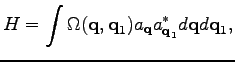
![$\displaystyle H_f=\int \check{a}_{\textbf{k}\textbf{x}} [\omega _{\textbf{k}\te...
...k}\textbf{x}},\cdot\}]\check{a}_{\textbf{k}\textbf{x}}^*d\textbf{k}d\textbf{x},$](img110.png)