Introduction

In order to analyze the behavior of general nonlinear system, the first necessary step is to analyze the linear system. The classical examples are finite dimensional Hamiltonian systems with coupled degrees of freedom. The dynamical behavior of such systems for small excitations, is determined by the form of the quadratic part of their Hamiltonians, which correspond to the linear dynamics. A detailed classification of the canonical normal forms for such Hamiltonians was given by Galin and it was summarized in one of the appendices of Arnold's book [1]. Another class of examples of nonlinear systems, which behavior crucially depends on the linear part, is weakly interacting dispersive waves in continuous media that are studied in Wave Turbulence (WT). These systems often have analogs among discrete systems, e.g. a chain of coupled oscillators, and correspondingly their quadratic Hamiltonians have analogs among Galin-Arnold canonical forms. Examples where WT has important applications are surface gravity waves [2], $\beta$ -plane turbulence in oceans and atmospheres [3,4], internal waves in the ocean [5], weak MHD turbulence [6], Bose-Einstein condensate [7,8] and plasmas [9]. Traditionally, WT theory is applied to homogeneous systems. The linear interaction Hamiltonian describing such homogeneous systems is given by [10]

$$H_2=\int\left( A_\textbf{k}\vert a_\textbf{k}\vert^2d\textbf{k}+\... ...{-\textbf{k}}+B_\textbf{k}^*a_\textbf{k}^*a_{-\textbf{k}}^*)\right)d\textbf{k},$$ (1)

where $a_\textbf{k}$ is a complex-valued field, the bold face denotes a $d$ dimensional vector in $\mathbb{R}^d$ . The linear canonical transformation to the new variables $b_\textbf{k}$ that was first used by Bogolyubov in 1958 for the system of fermions, brings this Hamiltonian to its normal form

$$H_2=\int\omega _\textbf{k}\vert b_\textbf{k}\vert^2d\textbf{k},$$ (2)

where $\omega _\textbf{k}$ is a linear dispersive relationship. The formalism of WT significantly enhanced our understanding of spectral energy transfer in ocean, atmosphere, plasma, other system of nonlinear waves [10]. Wave turbulence deals with weakly nonlinear waves with quasi-random phases. Using WT, one can derive a kinetic equation for the wave spectrum, which evolves due to resonant wave interactions.

In order for the resonant energy transfers to occur, certain resonance conditions need to be satisfied. In particular, for the systems dominated by three wave interactions, such as internal waves in the ocean or capillary waves [11], these conditions are given by

$$\omega _\textbf{k} = \omega _{\textbf{k}_1}+\omega _{\textbf{k}_2},$$

$$\textbf{k} = \textbf{k}_1+\textbf{k}_2.$$

Similar four-wave resonant conditions should be satisfied for the resonant interactions in the four-wave systems.

Often, WT is not spatially homogeneous and its statistical properties vary in space due to a trapping potential, inhomogeneous background density or an inhomogeneous velocity field. Examples of such systems are the Bose-Einstein Condensate (BEC) in the presence of a trapping potential [8] and an interaction of the long "aged" gravity waves with a swell [12]. In general, the idea is to consider a small amplitude high frequency perturbation of a large-scale solution of the dynamic equation (e.g. the condensate). The effects of this coordinate dependent background solution can most easily be understood using a wave-packet formalism. This formalism was first used to approximate the Schrödinger's wave function by a quasi-monochromatic wave by Wentzel [13], Kramers [14], and Brillouin [15]. Their initials give the term WKB approximation. The WKB approximation is applicable if the wavepacket wavelength $l$ is much shorter than the characteristic wavelength $L$ of a large scale solution

$$\epsilon=\frac{l}{L}\ll 1.$$

The essence of WKB approach is that the wave numbers, characterizing the wavepacket are the functions of coordinates. This is due to the distortion of the wave packets by the media, leading to a temporal wavenumber dependence. Such an effect may have a dramatic effect on nonlinear resonant wave interactions. Indeed, the resonant conditions (3) may now be satisfied only in a finite part of a domain, or for a particular wave packet, only for a finite time.

The goal of this paper is to use the spatially dependent WKB wave packets to find a canonical form for the quadratic Hamiltonian for the inhomogeneous systems. This problem can be considered as an extension of certain (oscillatory) members from the Galin-Arnold classification of quadratic forms onto the infinite-dimensional and continuous space. The physical motivation for such a formulation is that, since the Hamiltonian description is natural for WT in homogeneous systems, it lays down a necessary framework for generalization onto the inhomogeneous media.

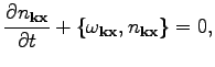
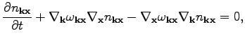
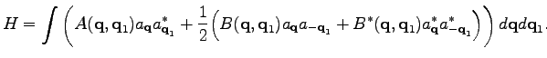
To begin, we write down the general Hamiltonian for the system of linear waves propagating in the inhomogeneous background. We will show in Section 2 that such general Hamiltonian for the variable $a_\textbf{q}$ is given by the following quadratic form:

$$H=\int \left(A(\textbf{q},\textbf{q}_1)a_\textbf{q}a^*_{\textbf{q... ...tbf{q}_1)a^*_\textbf{q}a^*_{-\textbf{q}_1}\Big)\right)d\textbf{q}d\textbf{q}_1.$$ (3)

The main result of the present paper is that this general Hamiltonian (4) can be transformed to the following canonical form

$$H=\int c_{\textbf{k}\textbf{x}}[\omega _{\textbf{k}\textbf{x}}-\t... ...\textbf{k}\textbf{x}},\cdot\}]c_{\textbf{k}\textbf{x}}^*d\textbf{k}d\textbf{x},$$ (4)

where $\omega _{\textbf{k}\textbf{x}}$ and $c_{\textbf{k}\textbf{x}}$ are the new position-dependent dispersion relationship and normal field-variable, correspondingly, and a Poisson bracket is defined by

$$\{f,g\}=\nabla_\textbf{k}f\cdot\nabla_\textbf{x}g-\nabla_\textbf{k}g\cdot\nabla_\textbf{x}f.$$

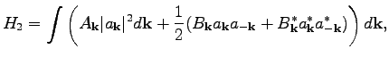
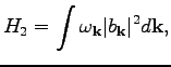
This novel canonical Hamiltonian is a generalization of the Hamiltonian (2) for the inhomogeneous systems. The approach used in the paper can be viewed as a generalization of the Bogolyubov transformation, which diagonalizes Hamiltonian (1) to the for (2) via canonical transformation. Similarly, Hamiltonian (4) can be transformed into the canonical form (5), however, now using near-canonical transformations. In the Hamiltonian (5), the second and the third terms in the brackets correspond to the higher order corrections to the dispersion relation due to the inhomogeneity. We prove that the Hamiltonian (4) can be transformed into a canonical form (5) in the case when the heterogeneity is weak. Formally, the requirement of weak inhomogeneity means that the coefficients $A(\textbf{q},\textbf{q}_1)$ and $B(\textbf{q},\textbf{q}_1)$ are strongly peaked at $\textbf{q}-\textbf{q}_1=0$ , i.e. $A(\textbf{q},\textbf{q}_1)=0$ for $\vert\textbf{q}-\textbf{q}_1\vert>\varepsilon$ for some small $\varepsilon$ . Based on this requirement, we derive below the re-normalized dispersion relationship and the transformation formulas from $a_\textbf{k}$ to $c_{\textbf{k}\textbf{x}}$ accurate up to the first order in $\varepsilon$ . It turns out that just Bogolyubov's transformation is not enough in this case. The phase coordinate systems should also be perturbed by a near-identity transformation in addition to the Bogolyubov's rotation. Then, the Hamiltonian becomes diagonal up to the first order in $\epsilon$ .

From the novel canonical form of the Hamiltonian given by Eq. (5), the traditional radiative action balance equation can easily be obtained:

$$\frac{\partial n_{\textbf{k}\textbf{x}}}{\partial t}+\nabla_\text... ...\omega _{\textbf{k}\textbf{x}}\nabla_{\textbf{k}}n_{\textbf{k}\textbf{x}}=0, %$$

or, shorter,

$$\frac{\partial n_{\textbf{k}\textbf{x}}}{\partial t}+\{\omega _{\textbf{k}\textbf{x}},n_{\textbf{k}\textbf{x}}\}=0,$$ (5)

where $n_{\textbf{k}\textbf{x}}$ denotes the ensemble average of the squared amplitude of the wave, i.e., $n_{\textbf{k}\textbf{x}}\equiv\langle \vert c_{\textbf{k}\textbf{x}}\vert^2\rangle$ . Equation (6) is now a standard equation which is used in statistical modeling of wave systems [16].

The paper is organized as follows. In Section 2, we give simple and instructive examples that motivate the study of inhomogeneous WKB systems. In Section 3, we introduce the window transforms and other formulas that we be extensively used later. In Section 4, we discuss the case of a nearly-diagonal Hamiltonian. We show how it can be transformed to a canonical form (2) and provide a couple of representative examples. In Section 5, we study the Hamiltonian in a general form (4). We present the series of near-canonical and near-identical transformations that bring the Hamiltonian (4) to the form (5). We also demonstrate the application of this approach to the nonlinear Schrodinger equation with the condensate. We end the paper with the concluding remarks.