Preliminaries

In this Section, we set up the stage for formulation of our results. Here, we give basic definitions, and obtain frequently used formulas.

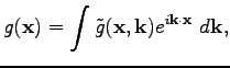
We use the following definition of direct and inverse Fourier transforms:

$$\hat{g}(\textbf{k}) = \frac{1}{(2\pi)^d}\int g(\textbf{x}) e^{-i\textbf{k}\cdot\textbf{x}}d \textbf{x},$$

$$g(\textbf{x}) = \int \hat{g}(\textbf{k})e^{i\textbf{k}\cdot\textbf{x}}d\textbf{k}.$$

Next, we generalize the Fourier transform to spatially inhomogeneous systems. In order to do that, we use a window transform of $g(\textbf{x})$ :

$$\Gamma[g(\textbf{x})]\equiv\tilde{g}(\textbf{x},\textbf{k}) = \fr... ...extbf{x}_0\vert)g(\textbf{x}_0)e^{-i\textbf{k}\cdot\textbf{x}_0}~d\textbf{x}_0.$$ (15)

Here, $f(x)$ is an arbitrary fast decaying at infinity window function. The parameter $\varepsilon^*$ is defined by the spatial scales of the inhomogeneity and the propagating wave-packets in the following manner. First, we introduce the characteristic length of inhomogeneity to be of the order $1/\varepsilon$ . Then, we take the width of the window, which is of the order $1/\varepsilon^*$ , to be much smaller than the characteristic length of inhomogeneity. On the other hand, the width of the window is chosen to be much larger than the wavelength of the waves that propagate in the inhomogeneous medium, which is of the order $1$ . Therefore, we have

$$\varepsilon \ll\varepsilon^*\ll 1.$$ (16)

The special case when $f(x)=\exp(-x^2)$ is called Gabor transform [17]. Note that, when $\varepsilon^*$ approaches zero, $f(\varepsilon^*x)$ approaches the constant function with the value one. Consequently, the Gabor transform becomes a Fourier transform. Therefore the Fourier transform can be seen as an averaging over an infinitely large window.

The inverse of the window transform (17) is given by

$$g(\textbf{x})=\int\tilde{g}(\textbf{x},\textbf{k})e^{i\textbf{k}\cdot\textbf{x}}~d\textbf{k},$$ (17)

where we have used $f(0)=1$ . We emphasize that Eq. (19) and all the formulas that we obtain below can be obtained using any fast decaying at infinity window function and are independent of the particular form of $f(x)$ as long as it is sufficiently smooth.

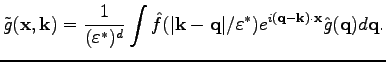
Now, we present the formulas for the window transform, which will be useful later. First, we express the window transform $\tilde{g}(\textbf{x},\textbf{k})$ in terms of the Fourier transform $\hat{g}(\textbf{k})$

$$\tilde{g}(\textbf{x},\textbf{k})=\frac{1}{(\varepsilon^*)^d}\int ... ...on^*)e^{i(\textbf{q}-\textbf{k})\cdot\textbf{x}}\hat{g}(\textbf{q})d\textbf{q}.$$ (18)

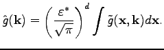
Next, we express the Fourier image $\hat{g}(\textbf{k})$ in terms of the window variable $\tilde{g}(\textbf{x},\textbf{k})$

$$\hat{g}(\textbf{k})=\left(\frac{\varepsilon^*}{\sqrt{\pi}}\right)^d\int\tilde{g}(\textbf{x},\textbf{k})d\textbf{x}.$$ (19)

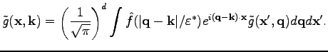
By combining Eqs. (20) and (21), we obtain the following formula

$$\tilde{g}(\textbf{x},\textbf{k})=\left(\frac{1}{\sqrt{\pi}}\right... ...bf{k})\cdot\textbf{x}}\tilde{g}(\textbf{x}',\textbf{q})d\textbf{q}d\textbf{x}'.$$ (20)

After introducing notations and formulas that will be extensively used below, we proceed to the discussion of the main results of the paper.