Next: Preliminaries
Up: Motivation
Previous: Three-wave case.
Four-wave systems are similar to three-wave systems when small scale
perturbations on the background of the large scale excitations are
considered. Indeed, we show below that the quadratic part of a
four-wave Hamiltonian of small scale perturbation has the form
(4). We start from a standard four-wave
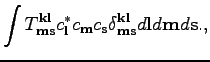
Hamiltonian [10]:
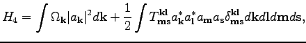 |
|
|
(11) |
where  is an interaction coefficient. The corresponding equation
of motion takes the form
is an interaction coefficient. The corresponding equation
of motion takes the form
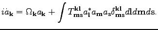 |
|
|
(12) |
We then consider a perturbed solution
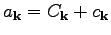 where
where
 is
a small-scale perturbation. Assuming that
is
a small-scale perturbation. Assuming that
 is an exact solution
to the equation of motion with Hamiltonian (13), we obtain
the following equation of motion for
is an exact solution
to the equation of motion with Hamiltonian (13), we obtain
the following equation of motion for
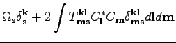
Since
is a known large scale solution, we obtain
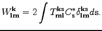
where we defined the kernels
 and
and
 as
as
and
The linear part of
equation (14) has the same form as the linear part of the
corresponding equation obtained for the three-wave
case (9). Thus, this linear part corresponds to the same
first two terms as in Hamiltonian (11). Note also
similarity of the quadratic terms in (9) and (14).
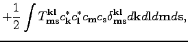
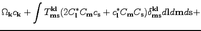
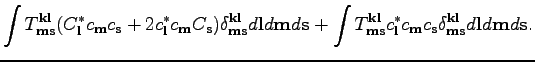
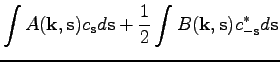
Note that (14) correspond to the following Hamiltonian
This appears to be a standard Hamiltonian for the inhomogeneous system
with four-wave interactions. Indeed, the quadratic part (first line)
of this Hamiltonian is the Hamiltonian
(4). Cubic term is the three-wave interactions
with the background large scale wave (i.e. four wave interaction where
the role of the fourth wave is assumed by the background wave). Notice
that unlike traditional three wave interactions in a homogeneous
environment, momentum is not conserved by this term. This is
the effect of breaking of spatial symmetry by an inhomogeneous
background. Lastly, the quartic term (third line) is the standard
four wave interactions Hamiltonian. We show in this paper that the
quadratic part of this Hamiltonian may be reduced to the novel canonical Hamiltonian for spatially inhomogeneous systems (5).
In this section we have demonstrated that if the general wave system
is dominated by three-wave or four-wave interactions, and consists of
short scale waves superimposed on known large-scale motion, its
quadratic Hamiltonian is given by the (4).
Next: Preliminaries
Up: Motivation
Previous: Three-wave case.
Dr Yuri V Lvov
2008-07-08
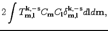
![$\displaystyle \int \left[ \frac{1}{2} W^{\textbf{k}}_{\textbf{l}\textbf{m}}c_\t...
...xtbf{k}\textbf{m}})^* c_\textbf{l}c_\textbf{m}^* \right] d\textbf{l}d\textbf{m}$](img61.png)
![$\displaystyle \int A(\textbf{k},\textbf{l})c_\textbf{l}c_\textbf{k}^*d\textbf{l...
...k},\textbf{l})c_{-\textbf{l}}^*c_\textbf{k}^*+c.c.\right]d\textbf{k}d\textbf{l}$](img71.png)
![$\displaystyle + \frac{1}{2}\int
[W^\textbf{k}_{\textbf{l}\textbf{m}}c_\textbf{k}^*c_\textbf{l}c_\textbf{m}+c.c.]d\textbf{k}d\textbf{l}d\textbf{m}+$](img72.png)