


Next: Estimation of the two-loop
Up: Statistical Description of Acoustic
Previous: Rules for writing and
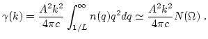
Let us start from (4.18) and
introduce
 with
with
 given by (4.14):
where
 |
(113) |
is ``triad-interaction'' frequency and
 is triad
interaction time. One can consider (B1 - B2) as an
integral equation for the damping of wave
is triad
interaction time. One can consider (B1 - B2) as an
integral equation for the damping of wave
 and for the frequency
 .
.
First we consider these equations in the limit of weak interaction
where,  , and the main contribution to the first term in
(B1) comes from the region where
, and the main contribution to the first term in
(B1) comes from the region where
 |
(114) |
These are conservation laws for 3-wave confluence processes  . The main contribution for the second term in (B1) comes
from the region
. The main contribution for the second term in (B1) comes
from the region
 |
(115) |
These are conservation laws for decays processes  . For weak
interaction one may replace in (4.2) and (4.3)
. For weak
interaction one may replace in (4.2) and (4.3)
 on
on
 . Than it follows from
(4.2) and (4.3) that
. Than it follows from
(4.2) and (4.3) that
 with
with
 directed along
  . This fact makes it natural to introduce in integrals (B1)
new variables: scale positive variable
. This fact makes it natural to introduce in integrals (B1)
new variables: scale positive variable  and two-dimensional
vector
and two-dimensional
vector  such that
 |
(116) |
In the first term of (B1)
 |
(117) |
In the second term
 |
(118) |
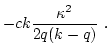
For  the denominators in integrals (B1) strongly
depend on
the denominators in integrals (B1) strongly
depend on  . Indeed:
This allows to neglect dependence of interaction
 and correlation
  in numerator of
(B1) for estimation. The result is
in numerator of
(B1) for estimation. The result is
where
 |
(122) |
is a factor in (2.20) so that for parallel or almost parallel
wavevectors
 . After
changing of variables this integral becomes to be more transparent:
. After
changing of variables this integral becomes to be more transparent:
One may estimate
 from the fact that
our expressions were obtained by expanding in
from the fact that
our expressions were obtained by expanding in  , therefore
should be at least
, therefore
should be at least  .
.
Now let us consider the imaginary and real part of  separately. It is convenient to begin with
:
separately. It is convenient to begin with
:
Here we changed the upper limit of integration:
 because the main contribution to the integral comes from the area
 . After trivial integration with respect of
  one has:
This expression for
 corresponds to that given by
the kinetic equation [1] for waves. For further progress it is
necessary to do some assumption about
corresponds to that given by
the kinetic equation [1] for waves. For further progress it is
necessary to do some assumption about  . Let us assume that
vanishes with growing of
. Let us assume that
vanishes with growing of  faster than
 .
.![[*]](file:/usr/share/latex2html/icons/footnote.png) For such
spectra the main contribution to the integral comes from small
For such
spectra the main contribution to the integral comes from small  . In this case contributions from first and second integrals in
(B14) coincides and may be represented in the form:
. In this case contributions from first and second integrals in
(B14) coincides and may be represented in the form:
 |
|
|
(126) |
In this case contributions from first and second integrals in
(B14) coincides and may be represented in the form:
|
|
|
(127) |
Next: Estimation of the two-loop
Up: Statistical Description of Acoustic
Previous: Rules for writing and
Dr Yuri V Lvov
2007-01-17
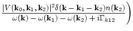
![$\displaystyle \Bigg(
\frac{\vert V({\bf k}_2,{\bf k},{\bf k}_1)\vert^2
\delta({...
..._2)\big]}
{\omega({\bf k})+\omega({\bf k}_1)
-\omega({\bf k}_2)+i\Gamma_{k12} }$](img482.png)

![$\displaystyle \frac{A^2k}{8\pi^2}\int_0^{k^2}d\kappa^2
\Bigg[ \int_0^\infty d q \frac{q(k+q)\big[n(q)-n(k+q)\big]}
{c k \kappa^2/[2q(k+q)]+i\Gamma_{k12}}$](img508.png)
![$\displaystyle \int_o^kd q \frac{q(k-q)n(q)} {-c k
\kappa^2/[2q(k-q)]+i\Gamma_{k12}}
\Bigg] \ ,$](img509.png)
![$\displaystyle \frac{[n(q)-n(k+q)]}{y+i\Gamma_{k12}}
-\int_0^{y_{\rm max}}
d y\int_o^k d q \frac{q^2(k-q)^2n(q)}{y-i\Gamma_{k12}}
\Bigg] \ .$](img513.png)
![$\displaystyle \frac{
\big[n(q)-n(k+q)\big]} {y^2+\Gamma_{k12}^2}
+ \int_0^k d q \frac{q^2(k-q)^2n(q)\Gamma_{k12}}{y^2+\Gamma^2_{k12}}
\Bigg] \ .$](img518.png)
![$\displaystyle \frac{A^2}{8\pi c }\Bigg[ \int_0^\infty
q^2(k+q)^2\big[n(q)-n(k+q)\big] d q$](img521.png)
![$\displaystyle + \int_0^k q^2(k-q)^2n(q) d q\Bigg] \ .$](img522.png)