


Next: Calculations of .
Up: One-loop approximation
Previous: One-loop approximation
In the one-loop approximation expression for
 has the form
 |
(79) |
where
 is given by (A1-A3). Our
goal here is to analyze these expressions in one-pole approximation,
by substituting in it ``one-pole''
is given by (A1-A3). Our
goal here is to analyze these expressions in one-pole approximation,
by substituting in it ``one-pole''
 and
and
 from (4.11) and (4.16). In the resulting
expression one can perform the integration over
from (4.11) and (4.16). In the resulting
expression one can perform the integration over  analytically.
The result is
analytically.
The result is
Next we introduce
 , with
 given by (4.14) and consider (4.18) in the limit
of small
given by (4.14) and consider (4.18) in the limit
of small  , which allows us to perform analytically
integrations over perpendicular components of wavevectors. The result
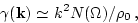
for the damping frequency
, which allows us to perform analytically
integrations over perpendicular components of wavevectors. The result
for the damping frequency  may be represented in the
following form (for details see Appendix B):
may be represented in the
following form (for details see Appendix B):
 |
|
|
(81) |
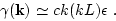
We introduced here cut-off for small  at
at  , where
  is the
size of the box. We also introduced ``the density of the number of
particles''
is the
size of the box. We also introduced ``the density of the number of
particles''  in the solid angle according to
 |
(82) |
such that the total number of particles
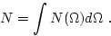 |
(83) |
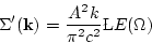
After substituting  from (B11), one has the following
estimate for
from (B11), one has the following
estimate for
 :
:
 |
(84) |
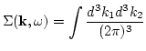
Consider now
 . It follows
from (B12) that
. It follows
from (B12) that
where
 is the
``triad interaction'' frequency. One may evaluate the integral with
respect to
is the
``triad interaction'' frequency. One may evaluate the integral with
respect to  as
as
 |
(86) |
After substituting
from (4.22), one has
 |
(87) |
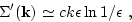
The main contribution to the integral (4.23) over  comes from
the infrared region
comes from
the infrared region  . It gives the estimate,
 |
(88) |
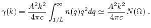
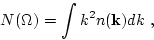
where we have defined the density of the wave energy in solid angle as
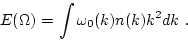 |
(89) |
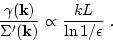
This value relates to as follows:
 |
(90) |
Equation (4.26) together with the expression (B11) for may
be written as
 |
(91) |
where
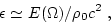 |
(92) |
is the dimensionless parameter of nonlinearity, the ratio of energy of
acoustic turbulence and the density of thermal energy of media
 , where
  is the concentration of
atoms.
is the concentration of
atoms.
Equation (4.22) for
may be written
in a similar form
 |
(93) |
One can see that
 |
(94) |
It means that for large enough inertial interval
 |
(95) |
and one may neglect the nonlinear corrections
 to
the frequency with respect to the damping of the waves
. That shows that our above calculations of
to
the frequency with respect to the damping of the waves
. That shows that our above calculations of
 is
self-consistent. Later we also will take into account only damping
in the expressions for the Green's functions taking
is
self-consistent. Later we also will take into account only damping
in the expressions for the Green's functions taking
 .
.
Next: Calculations of .
Up: One-loop approximation
Previous: One-loop approximation
Dr Yuri V Lvov
2007-01-17
![$\displaystyle \Bigg( \frac{\vert V({\bf k}_2,{\bf k},{\bf k}_1)\vert^2
\delta({...
..._2)\big]}
{\omega+\omega({\bf k}_1)-\omega({\bf k}_2)
+i ( \gamma_1+ \gamma_2)}$](img391.png)
![$\displaystyle \frac{A^2 k } { \pi^2 c^2}\int d q \int_0^{y_{\rm max}}
\frac{y d y }{y^2 + \Gamma_{k12}^2}
\left[ c q^3 n(q) \right] \,,$](img410.png)