The Green's function

We have assumed from the beginning, that the wave amplitude is small. Therefore,

$$\Sigma({\bf k},\omega)\ll\omega_0(k)\ .$$ (71)

As a result the Green's function has a sharp peak in the vicinity of $\omega=c k$ and one may (as a first step in the analysis) neglect the $\omega$-dependence of $\Sigma ({\bf k},\omega )$ and put

$$\Sigma({\bf k},\omega)\simeq\Sigma({\bf k},\omega\simeq c {\bf k}) \ .$$ (72)

The validity of this assumption will be checked later. Under this assumption the Green's function (4.2) has a simple one-pole structure:

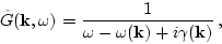$$\tilde G({\bf k},\omega) = \frac{1}{\omega-\omega({\bf k}) +i \gamma({\bf k})}\,,$$ (73)

where

$$\omega({\bf k}) = \omega_0({\bf k}) +{\rm Re}\Sigma({\bf k},\omega_*)\,,$$ (74)

$$\gamma({\bf k}) = -{\rm Im}\Sigma({\bf k},\omega_*)\ .$$ (75)

Now we have to decide how to choose $\omega_*$ ``in the best way''. The simplest way is to put $\omega_*=\omega_0({\bf k})=c k$, as it was stated in (4.10). As a next step we can take ``more accurate'' expression $\omega_*=\omega({\bf k})$, i.e. to take into account the real part of correction to $\omega_0({\bf k})$. But later we will see, that better choice is

$$\omega_*=\omega({\bf k})+i \gamma({\bf k})$$ (76)

which is consistent with the position of the pole of $\tilde G_*({\bf k},\omega)$. We will show that this choice is self consistent while deriving the balance equation in section 5.3.