Estimation of the two-loop diagrams.

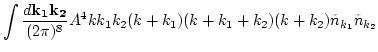
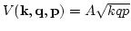
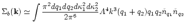
Let us write down analytical expression which correspond to one of the diagrams (b) in Fig.1(b)

$$\Sigma_b({\bf k},\omega) = \int \frac{ d{\bf k_1} d {\bf k_2} d\omega_1 d\omega_2} {(2\pi)^8} V_a V_b V_c V_d n(k_1,\omega_1)n(k_2,\omega_2)$$

$$\times G({\bf k_1}+{\bf k_2}, \omega_1+\omega_2) G({\bf k}+{\bf k_1}+ {\bf k_2},\omega+\omega_1+\omega_2)$$

$$\times G({\bf k}+{\bf k},\omega+\omega_2)$$ (128)

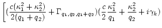
where $V_a, V_b, V_c, V_d$ are vertices,

$$V_a=V({\bf k_1}+{\bf k_2}+{\bf k},{\bf k},{\bf k_1}+{\bf k_2}),$$ (129)

$$V_b=V({\bf k_1}+{\bf k_2}+{\bf k},{\bf k_1},{\bf k}+{\bf k_2}),$$ (130)

$$V_c=V({\bf k_2}+{\bf k},{\bf k_2},{\bf k}),$$ (131)

$$V_d=V({\bf k_1}+{\bf k_2},{\bf k_1},{\bf k_2})$$ (132)

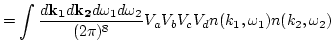
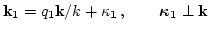
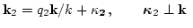
We just followed the rules of DT and integrated over all delta-functions. From now, the analyses will be parallel to that of appendix B. Let us use (4.16) for $n(k,\omega)$ and (4.11) for $G(k,\omega)$. Now we can easily perform integration over $\omega_1$ and $\omega_2$. Now, as it was done in appendix B, introduce $\Sigma_b({\bf k})=\Sigma_b({\bf k},\omega_*)$. Since all interacting wavevectors are almost parallel, we introduce two-dimensional vectors $\bf\kappa_1$ and $\bf\kappa_2$ such that

$${\bf k}_1=q_1 {\bf k} /k +{\bf\kappa_1 }\,, \qquad {\bbox \kappa_1 }\perp{\bf k}\$$ (133)

$${\bf k}_2=q_2 {\bf k} /k +{\bf\kappa_2 }\,, \qquad {\bbox \kappa_2 }\perp{\bf k}\$$ (134)

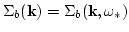
We use $V({\bf k}, {\bf q},{\bf p}) =A\sqrt{k q p}$. Since $\kappa_i\ll k$, we can expand resonance denominators in (C1) with respect to $\kappa_i$. The integrals will be dominated by regions, where $q_i\ll k$. By putting everything together, one gets

$$\Sigma_b({\bf k})\simeq \int \frac{ \pi^2 d q_1 d q_2 d \kappa_1^2 d \kappa_2^2}{2\pi^6} A^4 k^3 (q_1+q_2) q_1 q_2 \tilde n_{q_1} \tilde n_{q_2}$$ (135)

$$\left[ (\frac{c(\kappa_1^2+\kappa_2^2)}{2(q_1+q_2)}+ \Gamma_{q_1,... ... (\frac{c}{2} \frac{\kappa_1^2}{q_1}+\frac{\kappa_2^2}{q_2} +i\gamma_k) \right.$$

$$\left. (\frac{c \kappa_2^2}{2 q_2}+ i \gamma_k)\right]^{-1}$$ (136)

Substituting $\tilde n_q=n/q^{-9/2}$ we see, that indeed, the dominant part comes from the region of small $q_i$. We can estimate all these integrals to get

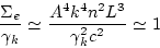
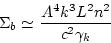$$\Sigma_b\simeq \frac{A^4 k^3 L^2 n^2}{c^2 \gamma_k}$$ (137)

where we used the small $q$ cutoff $1/L$. Finally

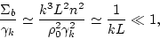$$\frac{\Sigma_b}{\gamma_k}\simeq \frac{k^3 L^2 n^2}{\rho_0^2 \gamma_k^2} \simeq\frac{1}{k L}\ll 1,$$ (138)

and we conclude, that contribution from diagrams of type (b) on Fig.1(b) is much less, than contribution from one-loop diagrams. But this is not the end of the story. Let us try to estimate contributions from diagrams of type (e) on Fig.1(b). Following the same guidelines, we obtain

$$\Sigma_e({\bf k})= \int {\frac{d {\bf k_1} {\bf k_2}}{(2 \pi)^8} A^4 k k_1 k_2 (k+k_1) (k+k_1+k_2)(k+k_2) \tilde n_{k_1} \tilde n_{k_2}}$$

$$\times \left[ (\omega_k+\omega_{k_1} -\omega_{k+k_1} + i\Gamma_{k,k_1,k+k_1}) \right.$$

$$\left.\times (\omega_k+\omega_{k_1}+\omega_{k_2} -\omega_{k+k_1+k_2} + i\Gamma_{k,k_1,k_2,k+k_1+k_2}) \right.$$

$$\times\left. (\omega_k+\omega_{k_2} -\omega_{k+k_2} + i\Gamma_{k,k_1,k+k_2})\right]^{-1}$$

Let us again introduce $\kappa_1$ and $\kappa_2$ as above, and substituting $\tilde n_q=n/q^{-9/2}$ we obtain the following estimation:

$$\frac{\Sigma_e}{\gamma_k}\simeq \frac{A^4 k^4 n^2 L^3}{\gamma_k^2 c^2 }\simeq 1$$ (139)

Therefore we conclude, that contribution from two loop diagrams is dominated by planar diagrams and of the order of one loop diagrams contribution.