Five-wave interaction on resonant surface

To find $T^{k k_1 k_2}_{k_3 k_4}$ one can calculate the terms of the order of $b^3$ and $b^4$ in the canonical transformation (4.2). This very cumbersome procedure was fulfilled by V.Krasitskii[7]. This is a kind of feat, but the resulting formulae are so complicated that hardly can be used for any practical purpose. In this article we offer much more simple and clear way to $T^{k k_1 k_2}_{k_3 k_4}$ involving a Feinman's diagram technique for the scattering matrix.

Our intermediate formulae are very complicated also, due to one-to-one correspondense of each term in the expression to a certain graphic picture, however all the procedure is much easy controlled. It is very remarkable that our final formula is very simple.

First we introduce so called formal classical scattering matrix. Let

$$H = H_2 + H_{int}$$

is a Hamiltonian of a some nonlinear system in a homogeneous space. Here 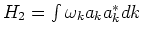$H_2 = \int \omega_k a_k a^*_k dk$, and $H_{int}$ is in general case an infinite series in power $a_k, a^*_k$

$$H_{int} = H_3 + H_4 + \ldots$$

The motion equation is as usual

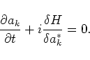$$\frac{\partial a_k}{\partial t} + i\frac{\delta H}{\delta a_k^*}=0.$$ (5.1)

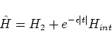
One can change $H$ to the auxiliary Hamiltonian

$$\nonumber \hat H = H_2 + e^{-\epsilon \vert t\vert} H_{int}$$

Now the equation (5.1) becomes linear at $t \rightarrow \pm \infty$ and

$$a_k(t) \rightarrow c^{\pm}_ke^{-i\omega_k t} \cr t$$

The asymptotic states $c^{\pm}_k$ are not independent, and actually

$$c^{+}_k = \hat S_{\epsilon}[c^{-}_k]$$

$\hat S_{\epsilon}[c^{-}_k]$ is a nonlinear operator which can be presented as a series in power of $c^{-}, {c^{-}}^{*}$. We will treat this series as formal one and will not care about their convergence. A formal series which is a result of the limiting transition

$$\hat S[c^{-}_k] = \lim_{\epsilon\to0}{\hat S_{\epsilon}[c^{-}_k]}$$

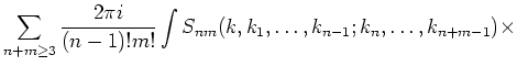
is the formal classic scattering matrix. It has the following form

$$\hat S[c^{-}_k] = c^{-}_k - \sum_{n+m\ge3}^{} \frac{2\pi i}{(n-1)!m!}\int S_{n m}(k,k_1,\ldots,k_{n-1};k_n,\ldots,k_{n+m-1})\times\cr$$ (5.2)

The functions $S_{n m}$ are the elements of the scattering matrix. They are defined on the resonant manifolds

$$k+k_1+\ldots +k_{n-1} = k_n+\ldots +k_{n+m-1}\cr \omega_k+\omega_{k_1}+\ldots +\omega_{k_{n-1}}$$ (5.3)

Two basic properties of the matrix elemets are important for us.

1. The value of the matrix element $S_{n m}$ on the resonant manifold (5.4) is invariant with respect to canonical transformation (4.2).
2. There is a simple algorythm for calculation of the matrix elements. The element $S_{n m}$ is a finite sum of terms which can be expressed through the coefficients of the Hamiltonians $H_i, i\le {n+m}$. Each term can be marked by a certain Feinman's diagram, having no internal loops. The rules of correspondense are described in the Appendix B.

Actually the classical scattering matrix is nothing but the Feinman's scattering matrix taken in the 'tree' approximation. This approximation makes a number of terms being finite for any element.

Our idea how to find $T^{k k_1 k_2}_{k_3 k_4}$ is the follow. We calculate first nonzero elements of the scattering matrix for the Hamiltonian (3.1) and for the Hamiltonian (4.1). Because of these two Hamiltonians are connected by the canonical transformation (4.2), the results must coinside. For surface gravity waves first nontrivial matrix element is $S_{2 2}$. In terms of the Hamiltonian (4.1) it is

$$S_{2 2}(k,k_1,k_2,k_3) = T^{k k_1}_{k_2 k_3}$$

Being calculated for the Hamiltinian (3.1), this element consist of six terms. They are presented (together with corresponding diagrams) in the Appendix B. One can see that the result coinside with the expression (4.3) on the resonant manifold (1.1).

In one-dimensional case the first integral in (5.3) can be calculated so that the first two terms in (5.3) has a form

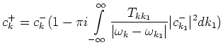$$c^+_k = c^-_k (1 - \pi i\int_{-\infty}^{\infty} \frac{T_{k k_1}}{\vert\omega_k - \omega_{k_1}\vert}\vert c^-_{k_1}\vert^2 dk_1)$$ (5.4)

This formula one more time stresses the fact that four-wave nonlinear processes in one-dimensional case lead only to the trivial scattering which does not produce ``new wave vectors''. The integral in (5.5) diverges logarithmically. It is why our scattering matrix is ``formal''. In reality in the one dimensional case the waves don't became a linear indeed if $t\to \infty$. They acquire logarithmically growing phase (see Zakharov, Manakov [13]).

The first nontrivial element of the scattering matrix in the one-dimensional case is

$$S_{3 2}(k,k_1,k_2,k_3,k_4) = T^{k k_1 k_2}_{k_3 k_4}$$

Being calculated in terms of the initial Hamiltonian (3.1) it consists of 81 terms. Their expressions together with diagrams are presented in the Appendix C.

In spite of complexity of the expression for $T^{k k_1 k_2}_{k_3 k_4}$ it can be enormousely simplified on the resonant manifold. We will discuss here only the case when all $k_i$ in the resonat conditions

$$k + k_1 + k_2 = k_3 + k_4 \cr \omega_{k} + \omega_{k_1} + \omega_{k_2}$$ (5.5)

have the same sign.

The manifold (5.6) can be parametrised as follow

$$k = a (p^2 - q^2 +1 - 2p)^2,\cr k_1$$ (5.6)

here $0 < \vert p\vert,\vert q\vert < 1, \vert p\pm q\vert < 1, a > 0$. Easy to see that $k_i$ here satisfy the inequality:

$$k, k_1 < k_3, k_4 < k_2$$

Plugging the parametrization (5.7) in the expression obtained for $T^{k k_1 k_2}_{k_3 k_4}$ we get a sum of more than thousands terms. Using the program for analytical calculations 'Mathematica' we manage to simplify this expression to the following form

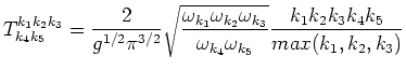$$T^{k_1 k_2 k_3}_{k_4 k_5} = \frac{2}{g^{1/2}\pi^{3/2}} \sqrt{\fra... ...{k_3}}{\omega_{k_4} \omega_{k_5}}} \frac{k_1 k_2 k_3 k_4 k_5}{max(k_1,k_2,k_3)}$$ (5.7)

This formula is the main result of the presented article. The fact that $T^{k k_1 k_2}_{k_3 k_4}\neq0$ on the resonant surface means that the system of gravity waves on a surface of deep water is nonintegrable Hamiltonian system.