Next: Five-wave interaction on resonant
Up: Five-wave interaction on the
Previous: Perturbation expansion for the
The Hamiltonian
 in the normal variables
  is too complicated to
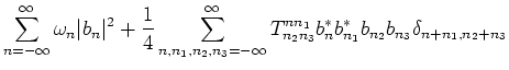
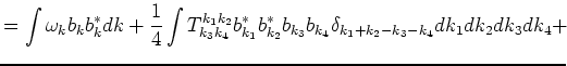
work with. Our purpose is to simplify the Hamiltonian to the form:
is too complicated to
work with. Our purpose is to simplify the Hamiltonian to the form:
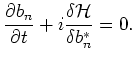
To do that we have to perform a transformation
(Zakharov, 1975 [9], Krasitskii, 1990 [10])
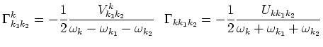
Here
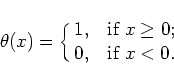
 is an arbitrary function
satisfying the conditions:
is an arbitrary function
satisfying the conditions:
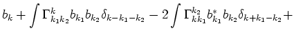
The transformation (4.2) is canonical up to
the terms of the order of  . It excludes from the Hamiltonian all
cubic terms. The form of the
. It excludes from the Hamiltonian all
cubic terms. The form of the
 depends on the choice
of the function
. Let first
depends on the choice
of the function
. Let first
 .
Then
.
Then
 and
and
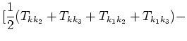
![$\displaystyle \hat T^{k k_1}_{k_2 k_3} = W^{k_1 k}_{k_2 k_3}- \hspace{9cm}\cr
-...
..._{k}+\omega_{k_1}}
+\frac{1}{\omega_{k_2+k_3}+\omega_{k_2}+\omega_{k_3}}\right]$](img134.png) |
|
|
(4.3) |
The expression (4.3) in spite of its complexity has
some remarkable properties. Let us consider all nontrivial solutions of the
equations (1.1). They consist of the manifold (1.5) and
of seven other manifolds which are obtained from (1.5) by
the permutations
Direct analytic calculation shows that
on all these manifolds. Recently Craig and Worfolk [14] confirmed this
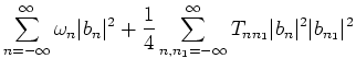
cancellation by the independent calculation. Another remarkable feature of
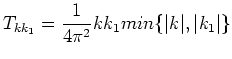
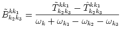
 is the simplicity of its diagonal part. Let us
denote
is the simplicity of its diagonal part. Let us
denote
A simple, but long calculation ([6], [11]) shows that
Let us consider the function
Obviously
Let us choose
One can check that this transformation makes replacement
of
by
 . So,
one can assume in future that
. So,
one can assume in future that
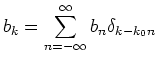
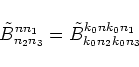
In the case of periodic boundary conditions
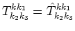
Introducing the notation
we can find that now
In the canonical transformation (4.2) all the
integrals are replaced now by the discrete sums. In particulary instead of
we have now
Let us choose
 |
|
|
(4.4) |
This expression has no singularities on the diagonals
 and
and
 . The transformation
(4.2) with (4.4) brings the Hamiltonian to
the Birghoff's form
. The transformation
(4.2) with (4.4) brings the Hamiltonian to
the Birghoff's form
This is a Hamiltonian of an integrable system. A level of
nonlinearity, allowing the representation (4.5) has to be studied
separately.
Next: Five-wave interaction on resonant
Up: Five-wave interaction on the
Previous: Perturbation expansion for the
Dr Yuri V Lvov
2007-01-17