Next: Example: an advection-type system
Up: The case of nearly-diagonal
Previous: Relation to the Wigner
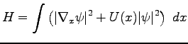
Consider a one-dimensional example of a linear Schrödinger equation
with a slowly varying potential. This equation is also referred to as
linearized Gross-Pitaevsky equation. It is used to describe a
formation of the BEC. It is given by
 |
|
|
(45) |
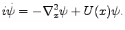
This equation can be written in a Hamiltonian form with the
Hamiltonian given by
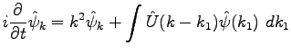
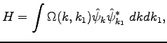
In the Fourier space, Eq. (49) becomes
with a corresponding Hamiltonian
where
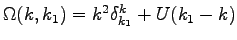 . Now we can apply
Lemma and find that the position dependent dispersion becomes
. Now we can apply
Lemma and find that the position dependent dispersion becomes
and the corresponding Hamiltonian in terms of Gabor variables takes
the canonical form (5):
![$\displaystyle H_f=\int \tilde{\psi}_{kx} [\omega_{kx}-x\nabla_x \omega_{kx}+i\{\omega_{kx},\cdot\}]\tilde{\psi}_{kx}^*dk dx.$](img195.png) |
|
|
(46) |
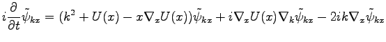
It follows from the Lemma that the Gabor variables provide a canonical
description of the system (49). Indeed, since
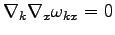 , we do not need to make a near-identity
transformation (41) in the Lemma. Therefore, it is instructive to obtain the
same result by directly applying Gabor transform to the both sides of
Eq. (49). We have
, we do not need to make a near-identity
transformation (41) in the Lemma. Therefore, it is instructive to obtain the
same result by directly applying Gabor transform to the both sides of
Eq. (49). We have
![$\displaystyle \Gamma[\nabla_x^2\psi]=\nabla_x^2\tilde{\psi}_{kx}+
2ik\nabla_x\t...
...-k^2\tilde{\psi}_{kx}\approx2ik\nabla_x\tilde{\psi}_{kx}
-k^2\tilde{\psi}_{kx}.$](img197.png) |
|
|
(47) |
To obtain this equation we have neglected the higher order derivative
of the Gabor variable, since it is a slowly varying in  . Next, we
use the linear expansion of the potential
. Next, we
use the linear expansion of the potential
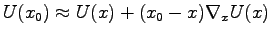 to find
![$\displaystyle \Gamma[U(x)\psi]=(U(x)-x\nabla_xU(x))\tilde{\psi}_{kx}+
i\nabla_xU(x)\nabla_k\tilde{\psi}_{kx}$](img200.png) |
|
|
(48) |
Combining Eq. (51) with Eq. (52), we obtain
And the corresponding Hamiltonian is given by Eq. (50).
Next: Example: an advection-type system
Up: The case of nearly-diagonal
Previous: Relation to the Wigner
Dr Yuri V Lvov
2008-07-08