Next: General case of waves
Up: The case of nearly-diagonal
Previous: Example: Linear Schrödinger equation
Let us consider an advection-type system. For simplicity of
calculations let us restrict our attention to a one dimensional case,
although a general dimensional case can also be considered. An
advection-type system has a Hamiltonian of the form
![$\displaystyle H=i\int U(x)\big[\psi(x)\nabla_x\psi^*(x)-\psi^*(x)\nabla_x\psi(x)\big]dx.$](img202.png) |
|
|
(49) |
with the corresponding equation of motion
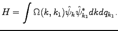
In the Fourier space, this system is described by the Hamiltonian
with the kernel
 |
|
|
(51) |
After applying Lemma to Hamiltonian (53), we obtain the
following canonical form
![$\displaystyle H_f=\int \check{\psi}_{kx} [\omega_{kx}-x\nabla_x \omega_{kx}+i\{\omega_{kx},\cdot\}]\check{\psi}_{kx}^*dk dx,$](img208.png) |
|
|
(52) |
where
 are the new variables.
 |
|
|
(53) |
is a position dependent frequency. Note that in this case we have
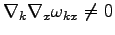 and the near-canonical change of
variables given by Eq. (41) had to be performed.
and the near-canonical change of
variables given by Eq. (41) had to be performed.
We can also obtain the same result by directly applying the Gabor
transform to Eq. (54).
Using the slow dependence of  on
on  (disregarding the second
derivative and higher), we obtain
(disregarding the second
derivative and higher), we obtain
![$\displaystyle \Gamma[U(x)\nabla_x\psi(x)]\approx$](img213.png) |
|
|
|
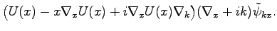 |
|
|
(54) |
Similarly, we have
![$\displaystyle \Gamma[\nabla_xU(x)\psi(x)]\approx\nabla_xU(x)\tilde{\psi}_{kx}.$](img215.png) |
|
|
(55) |
Substituting Eqs. (58) and (59) into
Eq. (54), we obtain
Using Eq. (57), we rewrite Eq. (60) as
 |
|
|
|
 |
|
|
(56) |
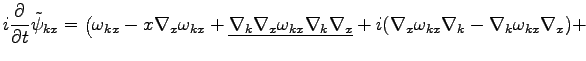
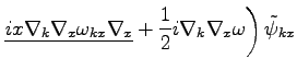
As in the Lemma, we neglect the higher order terms with the two
derivatives over
(underlined in Eq. (61)). In order
to obtain the canonical form of the equation of motion, we need to
make a near-canonical transformation
where  satisfies
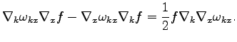 |
|
|
(57) |
For this special case, we obtain
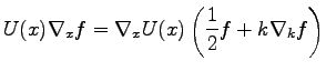 |
|
|
(58) |
We have to find the solution for Eq. (63) such that
 when
when
 . Therefore, we need to find a
solution in the form
. Therefore, we need to find a
solution in the form  , where
  satisfies
 .
Let us try to find a solution in the form
.
Let us try to find a solution in the form  , i.e., independent
of
, i.e., independent
of  . Then we have
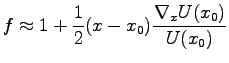
where  is an arbitrary constant. We expand
around some
point of reference
is an arbitrary constant. We expand
around some
point of reference  as
as
Let us choose the constant to be
 then we obtain
If
 and
and
 then
then
 and the transformation is near-canonical.
Next: General case of waves
Up: The case of nearly-diagonal
Previous: Example: Linear Schrödinger equation
Dr Yuri V Lvov
2008-07-08