Nonlinear Internal Waves in a Rotating Environment

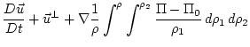
The equations for long internal waves in a rotating environment are particularly simple when written in the isopycnal coordinates $(x,y,\rho,t)$; they take the form in () with an extra term $\vec{u}^{\perp}$ due to the Coriolis force:

$$\frac{D \vec{u}}{D t} + \vec{u}^{\perp} + \nabla \frac{1}{\rho} \int^{\rho}\int^{\rho_2} \frac{\Pi-\Pi_0}{\rho_1} \, d\rho_1 \, d\rho_2 = 0,$$

$$\Pi_t + \nabla \cdot \left(\Pi\, \vec{u} \right) = 0\, .$$

where

$$\Pi_0 = \Pi_0(\rho)$$

is a reference stratification profile, that we introduce here for future convenience.

The expression for the potential vorticity in these coordinates is

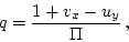$$q = \frac{1+v_x-u_y}{\Pi} \, ,$$ (25)

and it satisfies

$$\frac{Dq}{Dt} = 0 \, .$$ (26)

Notice that the advection of potential vorticity in () takes place exclusively along isopycnal surfaces. Therefore, an initial distribution of potential vorticity which is constant on isopycnals, though varying across them, will never change. Hence we shall propose that

$$q = q_0(\rho) \, ,$$ (27)

where $q_0(\rho)$ is an arbitrary function; i.e., one may assign any constant potential vorticity to each isopycnal surface. This is a highly nontrivial extension of the irrotational waves of the previous sections. Extending our description further to include general distributions of potential vorticity, varying even within surfaces of constant density, would necessarily complicate its Hamiltonian formulation, making it lose its natural simplicity. In fact, the problem of interaction between vorticity and waves is that of fully developed turbulence, which escapes the scope of our description. However, the ``pancake-like'' distributions of potential vorticity that we propose are common in stratified fluids, particularly the ocean and the atmosphere. They arise due to the sharp contrast between the magnitudes of the turbulent diffusion along and across isopycnals. Thus potential vorticity is much more rapidly homogenized along isopycnals than vertically, yielding the ``pancakes''. As we show below, even waves super-imposed on such a general and realistic distribution of potential vorticity admit a rather simple Hamiltonian description.

In order to isolate the wave dynamics satisfying the constraint (), we decompose the flow into a potential and a divergence-free part as in (). In terms of the potentials $\phi$ and $\psi$, () and () yield

$$1 + \Delta \psi = q_0 \Pi \, ,\nonumber$$

and, repeating the same steps as in nonlinear rotating shallow waters, the equations in () reduce to the pair

$$\Pi_t + \nabla \cdot \left(\Pi\, \left(\nabla \phi + \nabla^{{\perp}} \Delta^{-1} \left(q_0 \Pi-1\right)\right)\right) = 0\, ,$$

$$\phi_t + \frac{1}{2} \left\vert\nabla\phi+ \nabla^{{\perp}}\Delta^{-1} \left(q_0 \Pi-1\right) \right\vert^2$$

$$+ \Delta^{-1} \nabla \cdot \left[ q_0 \Pi \, \left(\nabla^{{\perp}}\phi - \nabla\Delta^{-1}\left(q_0 \Pi-1\right)\right) \right]$$

$$+ \frac{1}{\rho} \int^{\rho}\int^{\rho_2} \frac{\Pi-\Pi_0}{\rho_1} \, d\rho_1 \, d\rho_2 = 0\, .$$

This pair is Hamiltonian, with conjugated variables $\phi$ and $\Pi$, i.e. it can be written as

$$\Pi_t=\frac{\delta {{\cal H}}}{\delta \phi}, \ \ \ \ \ \ \ \phi_t=-\frac{\delta {{\cal H}}}{\delta \Pi} \, .\nonumber$$

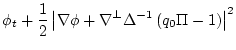
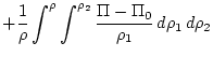
where the Hamiltonian is given by

$${\cal H}= \int \left[ \frac{1}{2} \Pi \, \left\vert\nabla... ...rho_1} \, d\rho_1\right\vert^2 \right] d\rho d\vec{r} \, .$$ (28)

Again, this Hamiltonian represents the sum of the kinetic and potential energy of the flow.

Notice the similarity of our description of internal waves with the Hamiltonian formulation for free-surface waves introduced by Zakharov in [31] and later by Miles in [32]. There, it was shown that the free-surface displacement and the three-dimensional velocity potential evaluated at the free surface are canonical conjugate variables. In our case, the canonical conjugate variables are also a displacement and a velocity potential, though the velocity potential in () is for the two-dimensional flow along isopycnal surfaces, and the displacement is the relative distance between neighboring isopycnal surfaces, as described above.

Looking back, we could have included some vorticity from early on; there was no need to take it equal to zero, as the last section shows. For shallow waters, it could have been any constant; for internal waves, any function of the density. It is clear though that, if one wanted to include arbitrary vorticity distributions, one would need to go fully Lagrangian, to exploit the fact that vorticity is preserved along particle paths. This would make the Hamiltonian structure less appealingly simple.

The key steps taken here for finding a simple Hamiltonian structure for internal waves, could be summarized as follows:

1. To consider long waves in hydrostatic balance. This, together with the choice of isopycnal coordinates, leads to a system of equations formally equivalent to an infinite collection of coupled shallow-water systems. This analogy allows us to generalize the relatively simple Hamiltonian structure of irrotational shallow-waters to the richer domain of internal waves.

2. To decouple waves from vorticity, by assuming the latter to be either zero, constant or uniform along isopycnal surfaces, with an arbitrary dependence on depth. This is facilitated by the choice of a flow description in isopycnal coordinates.

3. To realize that the potential $\phi$ is a good candidate canonical variable, and that its conjugate is the height $h$ for shallow waters, and the surrogate $\Pi$ for density in the isopycnal formulation of internal waves.

4. To introduce nonlocal operators into the Hamiltonian. These arise naturally from the ``elliptic'' constraints of hydrostatic balance and layered potential vorticity. Despite its unusual look, the Hamiltonian is invariably just the sum of the standard kinetic and potential energies, integrated over the domain.

The assumptions of hydrostatic balance and horizontally uniform background vorticity and shear, which simplify notoriously the description of the flows, are quite realistic for a wide range of ocean waves.