In this section, we apply the formalism of wave turbulence theory to derive a kinetic equation, describing the time evolution of the energy spectrum of internal waves. In order to do this, we need to assume that the waves are weakly nonlinear perturbations of a background state. In principle, we could adopt for this state an arbitrary background distribution of (layered) potential vorticity, vertical shear and stratification. To make the derivation clear, however, we focus here on the case with zero shear and zero potential vorticity, and a stratification profile with constant buoyancy frequency. Even though the mechanics for deriving the kinetic equation in the more general setting are entirely similar (though more cumbersome), the tools at our disposal for finding relevant exact solutions to these equations, are only applicable to the case with the simplest background.
To leading order in the perturbation, we obtain linear waves, with amplitudes modulated by the nonlinear interactions. These linear waves have, in general, a complex vertical structure (they are eigenfunctions of a differential eigenvalue problem), but reduce, in our case, to sines and cosines [33].
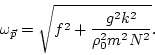
Let us now take (![]() ) and rewrite it in dimensional form:
) and rewrite it in dimensional form:
Here ![]() is the Coriolis parameter,
is the Coriolis parameter, ![]() is the acceleration due to
gravity. Note that
is the acceleration due to
gravity. Note that
The potential vorticity is, in dimensional form,
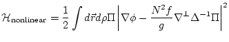
For the subsequent calculations it will be convenient to decompose the
potential ![]() into its equilibrium value and its deviation from
it. Therefore let us redefine
into its equilibrium value and its deviation from
it. Therefore let us redefine
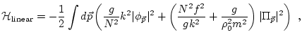
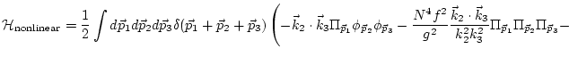
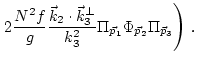
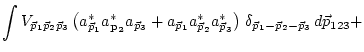
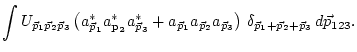
It can be represented as a sum of a quadratic and a cubic part:
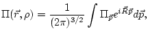
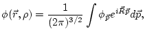
Let us use the Fourier transformation:
 |
|||
 |
|||
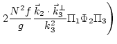
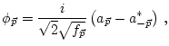
The canonical equations of motions (![]() ) form a pair of
real equations. Their Fourier transformation gives a pair of two
complex equations, yet not independent. To reduce this pair to one
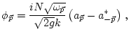
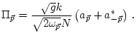
complex equation, one performs the transformation
) form a pair of
real equations. Their Fourier transformation gives a pair of two
complex equations, yet not independent. To reduce this pair to one
complex equation, one performs the transformation
This transformation turns the pair of canonical equation of motion
(![]() ) into a single equation for the complex variable
) into a single equation for the complex variable
![]() :
:
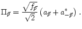
With such a choice of ![]() the transformations
(
the transformations
(![]() ) take the following form:
) take the following form:
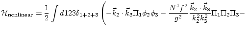
We would like to point out that the field equation
(![]() ) with the three-wave Hamiltonian
(
) with the three-wave Hamiltonian
(![]() ,
,![]() ,
,![]() ) are equivalent to the primitive equations of motion for internal waves
(
) are equivalent to the primitive equations of motion for internal waves
(![]() ) (up to the hydrostatic balance and Boussinesq
approximation); whereas the work reviewed in [10] instead
resorted to a small displacement approximation to arrive at similar
equations. We will argue elsewhere that this extra hypothesis, when
combined with an assumption of separation of scales, leads to the
questions of formal validity of small amplitude expansion observed in
([10]). Furthermore, our approach explicitly preserves all
the symmetries of the original primitive equations, like mass, energy
and potential vorticity conservation, as well as incompressibility,
whereas Lagrangian approaches based on small-displacement expansion
can only maintain approximate conservation of these symmetries.
) (up to the hydrostatic balance and Boussinesq
approximation); whereas the work reviewed in [10] instead
resorted to a small displacement approximation to arrive at similar
equations. We will argue elsewhere that this extra hypothesis, when
combined with an assumption of separation of scales, leads to the
questions of formal validity of small amplitude expansion observed in
([10]). Furthermore, our approach explicitly preserves all
the symmetries of the original primitive equations, like mass, energy
and potential vorticity conservation, as well as incompressibility,
whereas Lagrangian approaches based on small-displacement expansion
can only maintain approximate conservation of these symmetries.
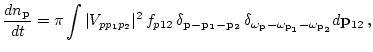
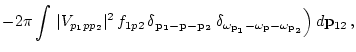
Following wave turbulence theory, one proposes a perturbation
expansion in the amplitude of the nonlinearity. This expansion gives
to leading order, linear waves. Then one allows the amplitude of the
waves to be slowly modulated by resonant nonlinear interactions. This
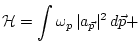
modulation is described by an approximate kinetic
equation [34] for the ``number of waves'' or wave-action
![]() , defined by
, defined by
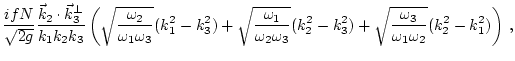
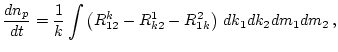
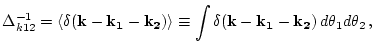
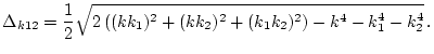
Assuming horizontal isotropy, one can average (![]() ) over
all horizontal angles, obtaining
) over
all horizontal angles, obtaining
![\begin{displaymath}
{\cal H}= \int \left[ \frac{1}{2} \Pi \,
\left\vert\nabla...
...ac{\Pi-\Pi_0}{\rho_1} \, d\rho_1\right\vert^2
\right] \, .
\end{displaymath}](img125.png)
![\begin{displaymath}
{\cal H}= \int d {\vec r} d \rho \left[ \frac{1}{2} \left( ...
...o} \frac{\Pi}{\rho_1} \, d\rho_1\right\vert^2
\right] \, .
\end{displaymath}](img134.png)
![$\displaystyle {\cal H}_{\rm linear}=
\int d {\vec r} d \rho
\left[ -\frac{g}{2 ...
...}
\left\vert\int^{\rho} \frac{\Pi}{\rho_1} \, d\rho_1\right\vert^2 \right] \, ,$](img136.png)