Nonlinear, Non-Rotating, Internal Waves

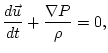
The non-dimensional equations of motion for long internal waves in an incompressible, stratified fluid with hydrostatic balance, are given by

$$\frac{d {\vec u}}{d t} + \frac{{\bf\nabla} P}{\rho} = 0, \ \ \ P_z+\rho = 0,$$

$$\frac{ d \rho}{d t} =0, \ \ \ {\bf\nabla}\cdot {\vec u} + w_z = 0 \, ,$$

where ${\vec u}$ and $w$ are the horizontal and vertical components of the velocity respectively, $P$ is the pressure, $\rho$ the density, $\nabla = (\partial_x, \partial_y)$ the horizontal gradient operator, and

$$\frac{d}{d t} = \frac{\partial}{\partial t} + {\vec u}\cdot{\bf\nabla} + w \frac{\partial}{\partial z}$$

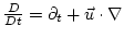
is the Lagrangian derivative following a particle.

Changing to isopycnal coordinates ($x,y,\rho,t$) , where the roles of the vertical coordinate $z$ and the density $\rho$ as independent and dependent variables are reversed, the equations become:

$$\frac{D \vec{u}}{D t} + \frac{\nabla M}{\rho} = 0\, ,$$

$$M_{\rho} = z \, ,$$

$$z_{\rho,t} + \nabla \cdot \left(z_{\rho} \vec{u} \right) = 0\, .$$

Here $\vec{u} = (u,v)$ is the horizontal component of the velocity field, $\nabla = (\partial_x, \partial_y)$ is the gradient operator along isopycnals, $\frac{D }{D t} = \partial_t + \vec{u} \cdot \nabla$, and $M$ is the Montgomery potential [30],

$$M=P+\rho\,z.$$

For flows which are irrotational along isopycnal surfaces, we introduce the velocity potential

$$\vec u=\nabla \phi.$$

Such a substitution allows us to integrate () once and eliminate $z$, after which these equations reduce to the pair

$$\phi_t + \frac{1}{2} \vert\nabla \phi\vert^2 + \frac{1}{\rho} \int^{\rho}\int^{\rho_2} \frac{\Pi}{\rho_1} \, d\rho_1 \, d\rho_2 = 0\, ,$$

$$\Pi_t + \nabla \cdot \left(\Pi\, \nabla \phi \right) = 0\, ,$$

where we have introduced the variable

$$\Pi = \rho M_{\rho \rho} = \rho z_{\rho}.$$

This variable $\Pi$ has at least two physical interpretations. One is that of density in isopycnal coordinates, since

$$\Pi \, d\rho = \rho \, dz \, .$$

The other is that of a measure of the stratification, namely the relative distance between neighboring isopycnal surfaces, since this distance $dz$ is given by

$$dz = \Pi \frac{d\rho}{\rho} \, .$$

Notice the similarity between () and the equations () for nonlinear shallow waters. Internal wave equations could be viewed as a system of infinitely many, coupled shallow water equations. This analogy allows us to identify a natural Hamiltonian structure for internal waves.

The variable $\Pi$ is also the canonical conjugate of $\phi$,

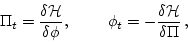$$\Pi_t=\frac{\delta {{\cal H}}}{\delta \phi}, \ \ \ \ \ \ \ \phi_t=-\frac{\delta {{\cal H}}}{\delta \Pi} \, ,$$ (9)

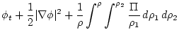
under the Hamiltonian flow given by

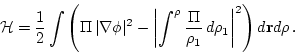$${\cal H}= \frac{1}{2}\int \left( \Pi \, \vert\nabla \phi\ve... ...}{\rho_1} \, d\rho_1\right\vert^2 \right) d {\bf r} d \rho\, .$$ (10)

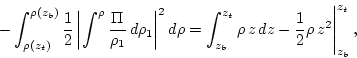
The first term in this Hamiltonian clearly corresponds to the kinetic energy of the flow; that the second term is in fact the potential energy follows from the simple calculation

$$\begin{eqnarray*} \frac{1}{2} \left\vert\int^{\rho} \frac{\Pi}{\rho_1} \, d\rho... ...rho \, z \, dz + d \left(\frac{1}{2} \rho\, z^2 \right) && \, , \end{eqnarray*}$$

so

$$-\int_{\rho(z_t)}^{\rho(z_b)} \frac{1}{2} \left\vert\int^{... ... \frac{1}{2} \rho\, z^2 \Bigg\vert _{z_b}^{z_t}\, , \nonumber$$

where $b$ and $t$ stand for bottom and top respectively, and the boundary conditions are usually such that the integrated term at the end is a constant.