The High Frequency Limit of the Kinetic Equations

The kinetic equation above describes general internal waves interacting in a rotating environment. However, as the frequency $\omega$ approaches the Coriolis parameter $f$, we also approach the scales where the ocean is actually forced. Hence the validity of the unforced kinetic equation in this range is questionable. Also, for small frequencies, the equations are strongly not scale invariant, which renders their analytical treatment more difficult. In this subsection, we shall concentrate on the high-frequency limit $\omega\gg f$, for which universality and scale invariance are more likely to develop. In fact, it is in this limit that we have found an exact steady solution in closed form in [20], and a family of solutions including the GM spectrum in [21]. Our reason for considering this limit again here is that we would like to write down the leading corrections brought about by the Coriolis term. It is highly plausible that these corrections will provide a clue to the selection process yielding the GM spectrum from the complete family of solutions to the non-rotating scenario.

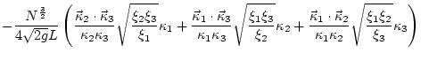
In the high frequency limit $\omega\gg f$, () becomes

$$\omega_{\bf p}\equiv \omega_{{\bf k},m} \simeq \frac{g}{N \rho_0} \frac{k}{\vert m\vert} \, ,$$

Furthermore, to leading order, the matrix element () retains only its first term, $I^1_{23}$. This is due to the fact that the second $J^1_{23}$ and third $K^1_{23}$ terms are proportional to $f ^2$ and $f$ respectively, and $f$ is negligible in the high frequency limit.

Indeed if one changes variables in () so that

$$\omega_i = N \xi_i,$$

rescaling the frequencies in terms of the buoyancy frequency $N$, and similarly one introduces

$$\vec k_i = \vec \kappa_i / L,$$

i.e. nondimensionalizing the horizontal wavevectors in terms of some distance $L$ to be determined, then

$$V^1_{23} = I^1_{23}+J^1_{23}+K^1_{23}$$

$$I^1_{23} = -\frac{N^{\frac{3}{2}}}{4\sqrt{2 g}L} \left( \frac{{\vec \kappa}_... ... \kappa}_2}{\kappa_1 \kappa_2}\sqrt{\frac{\xi_1 \xi_2}{\xi_3}} \kappa_3 \right)$$

$$J^1_{23} = \frac{N^{3/2}}{4 L\sqrt{ 2 g}} \frac{f^2}{N^2} \frac{1}{\sqrt{ 2 ... ...\frac{{\vec \kappa}_1\cdot{\vec \kappa}_2}{\kappa_1 \kappa_2}{\kappa_3} \right)$$

$$K^1_{23} = i\frac{N^{3/2}}{L \sqrt{2 g}}\frac{f}{N} \frac{{\vec \kappa}_2\cd... ...^2-\kappa_3^2) + \sqrt{\frac{\xi_3}{\xi_1\xi_2}}(\kappa_2^2-\kappa_1^2) \right)$$

Note that $K^1_{23}$ is proportional to $(f/N)$ and $J^1_{23}$ is proportional to $(f/N)^2$. Taking into account that, in the real ocean, $f/N\simeq 1/100$ we see that $J^1_{23}$ and $K^1_{23}$ term could safely be neglected from the matrix element in the high frequency limit.

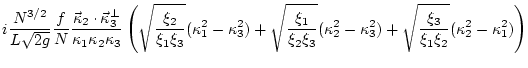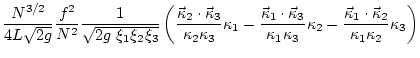
If one neglects both the $J^1_{23}$ and the $K^1_{23}$ terms, we arrive at the kinetic equation derived in [20] and studied further in [21], corresponding to a non-rotating environment.

If we assume that $n_{\bf p}$ is given by the power-law anisotropic distribution

$$n_{{\bf k},m}= k^x \vert m\vert^y \, ,$$ (38)

then the exponents $x$ and $y$ have to be such that () is a stationary solution to () in the high frequency limit. With the help of the Zakharov-Kuznetsov conformal mapping [31,39,43] it was shown in [20] that a particular choice, $x=-{7}/{2}, \ \ \ \ y=-{1}/{2} \, ,$ renders the right-hand side of () to be identical zero. Therefore the following wave action spectrum constitutes an exact steady state solution of ()

$$n_{{\bf k},m}= n_0\ \vert{\bf k}\vert^{-7/2} \vert m\vert^{-1/2};\$$ (39)

However, as pointed out in [34], the set of steady state solutions to the kinetic equation in cylindrical symmetry is not limited to one isolated point in $(x,y)$ space. This set corresponds instead to a curve in $(x,y)$ plane, where the collision integral surface $z=I(x,y)$ crosses a plane $z=0$. Such a curve for the internal wave kinetic equation was obtained in [21] by means of numerical integration of () for the set of power-law solutions ().

Remarkably, the high-frequency limit of the Garrett-Munk spectrum, $x=4,\ \ y=0$, turns out to be a member of this family of steady state solutions of the kinetic equation ().