Next: Three-wave case
Up: Wave Turbulence "Recent developments
Previous: Introduction
Setting the stage I: Dynamical Equations of motion
Wave turbulence formulation deals with a many-wave system with dispersion and
weak nonlinearity. For systematic
derivations one needs to start from Hamiltonian equation of motion.
Here we consider a system of weakly interacting waves in
a periodic box [1],
where  is often called the field variable. It represents the
amplitude of the interacting plane wave. The Hamiltonian is represented
as an expansion in powers of small amplitude,
is often called the field variable. It represents the
amplitude of the interacting plane wave. The Hamiltonian is represented
as an expansion in powers of small amplitude,
 |
(2) |
where  is a term proportional to product of
  amplitudes ,
where
 and
and
 are wavevectors on a
 -dimensional Fourier space lattice.
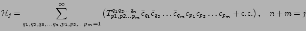
Such general -wave Hamiltonian describe the wave-wave interactions
where
-dimensional Fourier space lattice.
Such general -wave Hamiltonian describe the wave-wave interactions
where  waves collide to create
  waves. Here
 represents the amplitude of the
  process. In
this paper we are going to consider expansions of Hamiltonians up to
forth order in wave amplitude.
process. In
this paper we are going to consider expansions of Hamiltonians up to
forth order in wave amplitude.
Under rather general conditions the quadratic part of a Hamiltonian,
which correspond to a linear equation of motion, can be diagonalised
to the form
 |
(3) |
This form of Hamiltonian correspond to noninteracting (linear) waves.
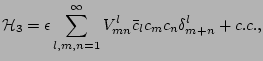
First correction to the quadratic Hamiltonian is a cubic
Hamiltonian, which describes the processes of decaying of single wave
into two waves or confluence of two waves into a single one. Such a Hamiltonian has the
form
where
 is a formal parameter corresponding to small
nonlinearity
(
is a formal parameter corresponding to small
nonlinearity
(  is proportional to the small amplitude whereas
  is
normalised so that
is
normalised so that
 .)
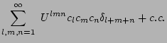
Most general form of three-wave Hamiltonian would also have terms describing the
confluence of three waves or spontaneous appearance of three waves out of vacuum. Such a
terms would have a form
It can be shown however that for systems that are dominated by three-wave
resonances such terms do not contribute to long term dynamics of systems.
We therefore choose to omit those terms.
.)
Most general form of three-wave Hamiltonian would also have terms describing the
confluence of three waves or spontaneous appearance of three waves out of vacuum. Such a
terms would have a form
It can be shown however that for systems that are dominated by three-wave
resonances such terms do not contribute to long term dynamics of systems.
We therefore choose to omit those terms.
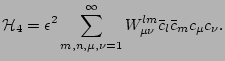
The most general four-wave Hamiltonian will have  ,
,  ,
,  ,
,  and
and  terms. Nevertheless , ,
and terms can be excluded from Hamiltonian by
appropriate canonical transformations, so that we limit our consideration to
only terms of
terms. Nevertheless , ,
and terms can be excluded from Hamiltonian by
appropriate canonical transformations, so that we limit our consideration to
only terms of
 , namely
It turns out that generically most of the weakly nonlinear systems can be
separated into two major classes: the ones dominated by three-wave
interactions, so that
 describes all the relevant dynamics
and
can be neglected, and the systems where the three-wave
resonance conditions cannot be satisfied, so that the
can be eliminated from a Hamiltonian by an appropriate
near-identical canonical transformation [25].
Consequently, for the purpose
of this paper we are going to neglect either
or
, and study the case of resonant three-wave or four-wave
interactions.
describes all the relevant dynamics
and
can be neglected, and the systems where the three-wave
resonance conditions cannot be satisfied, so that the
can be eliminated from a Hamiltonian by an appropriate
near-identical canonical transformation [25].
Consequently, for the purpose
of this paper we are going to neglect either
or
, and study the case of resonant three-wave or four-wave
interactions.
Examples of three-wave system include the water surface capillary waves,
internal waves in the ocean and Rossby waves. The most common examples of the four-wave
systems are the surface gravity waves and waves in the NLS model of nonlinear
optical systems and Bose-Einstein condensates.
For reference we will give expressions for the frequencies and the interaction
coefficients corresponding to these examples.
For the capillary waves we have [1,5],
 |
(4) |
and
![$\displaystyle V^l_{mn} = {1 \over 8 \pi \sqrt{2 \sigma}} (\omega_{l} \omega_m \...
...r ( k_l k_m)^{1/2} k_n } - {L_{k_l, -k_n} \over ( k_l k_n)^{1/2} k_m } \right],$](img39.png) |
(5) |
where
 |
(6) |
and  is the surface tension coefficient.
For the Rossby waves [13,14],
 |
(7) |
and
 |
(8) |
where  is the gradient of the Coriolis parameter and
  is the
Rossby deformation radius.
is the
Rossby deformation radius.
The simplest expressions correspond to the NLS waves [15,7],
 |
(9) |
The surface gravity waves are on the other extreme. The
frequency is
 but the matrix element is given by
notoriously long expressions which can be found in [1,17].
but the matrix element is given by
notoriously long expressions which can be found in [1,17].
Subsections
Next: Three-wave case
Up: Wave Turbulence "Recent developments
Previous: Introduction
Dr Yuri V Lvov
2007-01-23