Relations between Wave Amplitudes $a^+({\bf k}),\ \ a^-({\bf k})$ with Normal Variables of Acoustic Turbulence $b({\bf k}),\ b^*({\bf k})$.

Comparing Eqs. (2.4) and (2.5) we get

$$\delta\rho({\bf k},t) = \rho_0 \epsilon \Big\{ a^+({\bf k},t)\exp [i\omega({\bf k} ) t ]$$

$$+ a^-({\bf k},t)\exp [-i \omega({\bf k} ) t ]\Big\}(2\pi)^{3/2}$$ (46)

$$\Phi({\bf k},t) = \frac{i c^2 \epsilon }{ \omega({\bf k} ) } \Big\{a^+({\bf k},t) \exp[i\omega({\bf k} ) t]$$

$$- a^-({\bf k},t)\exp [-i \omega({\bf k} ) t ]\Big\}(2\pi)^{3/2}$$ (47)

Here $\Phi$ is velocity potential: ${\bf v} = \nabla \Phi$. This gives

$$a^{+}({\bf k},t) = \frac{\exp [-i\omega({\bf k}) t] } {2 \epsilon(2\pi)^{3/2} } \lef... ...bf k},t)\over \rho_0} -i \Phi({\bf k},t) \frac{\omega({\bf k})}{c^2 }\right]\,,$$

$$a^{-}({\bf k},t) = \frac{\exp [i\omega({\bf k}) t] }{2 \epsilon (2\pi)^{3/2} }\left[... ...a\rho({\bf k},t)\over \rho_0} + i \Phi({\bf k},t)\frac{\omega_k}{c^2}\right]\ .$$ (48)

Note, that $a^+$ and $a^-$ is dimensionless variables.

Now we can easily express $a^+({\bf k}),\ \ a^({\bf k})$ in terms of $b({\bf k}),\ b^*({\bf k})$ and thereby relate the two alternative approaches presented in this paper,

$$a^+({\bf k},t) = \frac{1}{ \epsilon }\sqrt{\frac{k}{2 c \rho_0}} (2\pi)^{-3/2}\exp [- i \omega({\bf k}) t] b^*({-\bf k})\,,$$ (49)

$$a^-({\bf k},t) = \frac{1}{ \epsilon }\sqrt{\frac{k}{2 c \rho_0}} (2\pi)^{-3/2}\exp [i \omega({\bf k}) t] b({\bf k})\ .$$ (50)

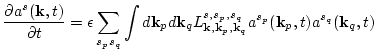
To check, that the two approaches are consistent, we rewrite the equation of motion (2.6) for $a_k^s$ neglecting $\epsilon^2$ (four-wave interaction) terms:

$$\frac{\partial a^s({\bf k}, t)}{\partial t}= \epsilon \sum_{s_p s... ...{{{\bf k}},{{\bf k}}_p,{{\bf k}}_q} a^{s_p} ({\bf k}_p, t) a^{s_q}({\bf k}_q,t)$$

$$\times \delta({\bf k}_p+{\bf k}_q - {\bf k} ) \exp\{i[ s_p\omega({\bf k}_p)+s_q\omega({\bf k}_q)- s \omega({\bf k} )]t\}$$

Now we substitute Eqs. (2.28) and (2.29) into (2.30) and obtain

$$\left[{\partial \over \partial t} + i \omega({\bf k})\right] b({{\bf k}},t)= -i \int d{\bf p} d{\bf q}\sqrt{\frac{k p q c }{4\pi^3\rho_0}}$$

$$\times \Big[ (\mu-2) +\cos{\theta_{{\bf k},{\bf p}}} +\cos{\theta_{{\bf k},{\bf q}}} +\cos{\theta_{{\bf p},{\bf q}}}\Big]$$ (51)

$$\times \left[\delta({{\bf k}+{\bf p}+{\bf q}})b_{{\bf p}}^*b_{{\bf q}}^*... ...*b_{{\bf q}} + \delta({{\bf k}-{\bf p}-{\bf q}})b_{{\bf p}} b_{{\bf q}} \right]$$

Now one can see that equation (2.31) looks exactly as (2.22) with Hamiltonian (2.19) and with coupling coefficient (2.20). Thus one conclude that the two approaches are equivalent and the choice between them is the question of taste.