Next: Hamiltonian Description of Acoustic
Up: Basic equation of motion
Previous: Basic equation of motion
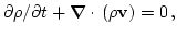
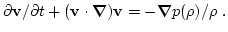
Consider the Euler equations for a compressible fluid:
| |
|
 |
|
| |
|
 |
(23) |
Here  is the Euler fluid velocity,
 the density, and
  is the pressure which, in the general
case, is a function of fluid density and specific entropy
is the pressure which, in the general
case, is a function of fluid density and specific entropy  [
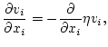
[ ]. In ideal fluids where there is no viscosity and heat
exchange, the entropy per unit volume is carried by the fluid, i.e.
obeys the equation
]. In ideal fluids where there is no viscosity and heat
exchange, the entropy per unit volume is carried by the fluid, i.e.
obeys the equation
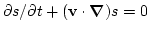 . A fluid in which the specific entropy is
constant throughout the volume is called barotropic; the pressure in
such fluid is a single-valued function of density
. A fluid in which the specific entropy is
constant throughout the volume is called barotropic; the pressure in
such fluid is a single-valued function of density  . In
this case,
. In
this case,
 may be expressed via the gradient of
specific enthalpy of unit mass
may be expressed via the gradient of
specific enthalpy of unit mass  and
and
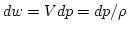 . Thus,
 .
.
Writing the fluid density
as
 , the velocity field as , the pressure field as
 and the enthalpy as
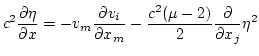
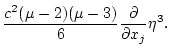
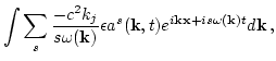
one can write (2.1) to third order in amplitude
in the following form
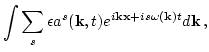
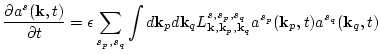
Let us introduce new variables as
where
 ,
,
 and
and  connotes summation over
  . From
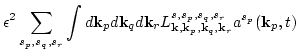
(2.2) and (2.3),
. From
(2.2) and (2.3),
where the summation is done over all signs of
 and we
used the shorthand notation
and we
used the shorthand notation
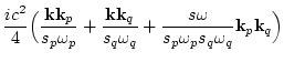
 . The coupling
coefficients are,
. The coupling
coefficients are,
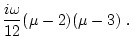
These coefficients have the following important properties:
where  . Note that if
 ,
the resonant manifold is not of codimension
one but degenerates to
,
the resonant manifold is not of codimension
one but degenerates to  , where
 ,
,
 . There are three cases.
- For
 ,
,
 ,
,
 ,
,
 ,
,  .
.
- For
 ,
,
 ,
,
 .
.
- For
 ,
,
,
,
 ,
,
 .
.
Next: Hamiltonian Description of Acoustic
Up: Basic equation of motion
Previous: Basic equation of motion
Dr Yuri V Lvov
2007-01-17