Next: Diagrammatic Approach to Acoustic
Up: Statistical Description of Acoustic
Previous: Relations between Wave Amplitudes
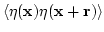
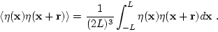
The analysis proceeds by first forming the hierarchy of equations for
the spectral cumulants (correlation functions of the wave amplitudes)
defined as follows. The mean is zero.
where
 denotes average and the presence of the
delta function is a direct reflection of spatial homogeneity. Indeed the
property of spatial homogeneity affords one a way of defining averages,
which does not depend on the presence of a joint distribution. We can
define the average
denotes average and the presence of the
delta function is a direct reflection of spatial homogeneity. Indeed the
property of spatial homogeneity affords one a way of defining averages,
which does not depend on the presence of a joint distribution. We can
define the average
 as
simply an average over the base coordinate, namely
as
simply an average over the base coordinate, namely
 |
(55) |
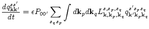
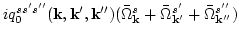
To derive the main results of this paper, it is sufficient to write the
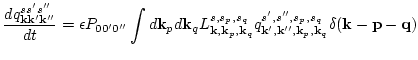
equations for the second and third order cumulants. They are
where the symbol  (
( ) means that we sum over all
replacements
) means that we sum over all
replacements
 (
(
 ).
).
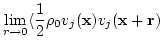
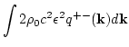
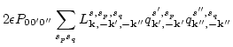
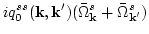
The total energy of the system per unite volume can be written as
since
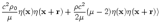
 . The spectral energy is
therefore
. The spectral energy is
therefore
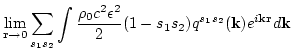
 . For convenience we
denote
. For convenience we
denote
 as
as  .
.
To leading order in  ,
,
 and
and
 (which we may call
 and
and
 ) are independent of time. Anticipating, however that
certain parts of the higher order iterates in their asymptotic
expansions may become unbounded, we will allow both
and
to
be slowly varying in time
) are independent of time. Anticipating, however that
certain parts of the higher order iterates in their asymptotic
expansions may become unbounded, we will allow both
and
to
be slowly varying in time
| |
|
 |
|
| |
|
 |
(59) |
and we will choose  and
and  to remove those terms with
unbounded growth from the later iteration. We will find that for
to remove those terms with
unbounded growth from the later iteration. We will find that for
 ,
,  is given by the right-hand side of acoustic KE:
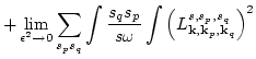
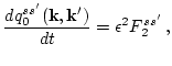
and that  and
and
 have the form
| |
|
 |
(60) |
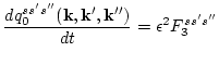
and
| |
|
 |
(61) |
respectively.
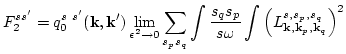
It is clear that
 can be interpreted as a complex
frequency modification. Its exact expression is given by
can be interpreted as a complex
frequency modification. Its exact expression is given by
and, when calculated out, is precisely equal to
 in (1.17). Note that in (3.11),
 and
and  is finite. The
 coefficient
comes from the term
coefficient
comes from the term  or
or
 in the asymptotic expansion. For finite , the dominant part is
.
in the asymptotic expansion. For finite , the dominant part is
.
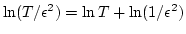
The perturbations method has the advantage that it is relatively simple
to execute. However, there is no a priori guarantee that terms
appearing later in the formal series cannot have time dependencies
which mean they affect the leading approximations on time scales
comparable to or less than  (e.g. a term
 should be accounted for before the term
  ). To check this,
one must have a systematic approach for exploring all orders in the
formal perturbation series and removing (renormalizing) in groups those
resonances which make their cumulative effects at time scales
). To check this,
one must have a systematic approach for exploring all orders in the
formal perturbation series and removing (renormalizing) in groups those
resonances which make their cumulative effects at time scales
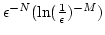 ,
,
 .
The diagram approach, which requires some familiarity to
execute, is designed to do this and, both for completeness and the
fact that we will have to proceed beyond the one-loop approximation to
resolve the questions of the angular redistribution of spectral
energy, we include it here.
.
The diagram approach, which requires some familiarity to
execute, is designed to do this and, both for completeness and the
fact that we will have to proceed beyond the one-loop approximation to
resolve the questions of the angular redistribution of spectral
energy, we include it here.
Next: Diagrammatic Approach to Acoustic
Up: Statistical Description of Acoustic
Previous: Relations between Wave Amplitudes
Dr Yuri V Lvov
2007-01-17