The basic ideas for writing down the kinetic equation to describe how weakly interacting waves share their energies go back to Peierls but the modern theories have their origin in the works of Hasselman [2], Benney and Saffmann [3], Kadomtsev [4], Zakharov [1], Benney and Newell [5,6]. A particularly important event in this history was the discovery of the pure Kolmogorov solution by Zakharov [7]. Usually, the thermodynamic equilibrium solutions can be seen from the kinetic equation by inspection. On the other hand, the solutions, corresponding to pure Kolmogorov spectra are much more subtle and only emerge after one has exploited scaling symmetries of the dispersion relation and the coupling coefficient via what is now called the Zakharov transformation[1].
But success to this point, namely the natural closure,
depended crucially on the fact the waves were
dispersive. This means that the group velocity is neither constant
in amplitude nor direction, or alternatively
stated, the dispersion tensor
Mathematically, these results are obtained by perturbation theory, in
which the terms leading to long time cumulative effects can be
identified, tabulated and summed. The method closely parallels that of
the Dyson-Wyld diagrammatic approach which will be discussed in
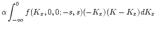
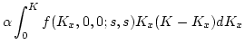
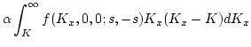
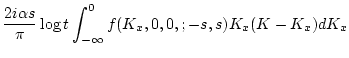
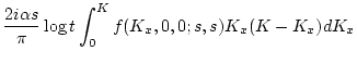
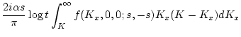
Section 4. A key part of the analysis is the asymptotic
(
![]() ) evaluation of
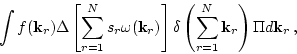
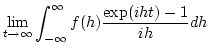
certain integrals such as
) evaluation of
certain integrals such as
But acoustic waves are not fully dispersive. The linear dispersion
relation,
While the extra term in (1.14) proportional to ![]() plays no
role in the spectral energy transfer, it will, however, appear in the
frequency modification.
Calculating the long time behavior of the higher order
cumulants leads to a natural re-normalization of the frequency,
plays no
role in the spectral energy transfer, it will, however, appear in the
frequency modification.
Calculating the long time behavior of the higher order
cumulants leads to a natural re-normalization of the frequency,
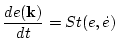
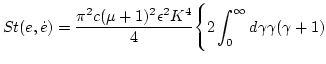
The equation (1.16) is nothing but a ``regular" kinetic equation
for the three-wave interactions, written in a dispersionless limit
![]() . In this case three wave resonant conditions
. In this case three wave resonant conditions
The derivation presented above is taken from the article of Newell and Aucoin [9], who made the first serious attempt of an analytical description of the dispersionless acoustic turbulence.
Newell and Aucoin [9] also argued that a natural asymptotic closure also obtains in two dimensions because of the relative higher asymptotic growth rates of terms in the kinetic equation involving only the spectral energy, but this is still a point of dispute, is not yet resolved and will not be addressed further here.
Independently the kinetic equation (1.16) was applied to acoustic
turbulence by Zakharov and Sagdeev [8] who used it just as a
plausible hypothesis. However, Zakharov and Sagdeev also suggested an
explicit expression for the spectrum of acoustic turbulence
Kadomtsev and Petviashvili [11] criticized this result on the
grounds that the kinetic equation is in the dispersionless case can
hardly be justified because of the special nature of the linear
dispersion relation. They suggested that acoustic turbulence in two
and three dimensions was much more likely to have parallels with its
analogue in one dimension. We have already mentioned in that case that
the usual statistical description is inadequate both because there is
no decorrelation dynamics and because shocks form no matter how weak
the nonlinearity initially is. The equilibrium statistics relevant in
that case is much more likely to be a random distribution of
discontinuities in the density and velocity fields which lead to an
energy distribution of (1.10). Further, Kadomtsev and
Petviashvili argued that even in two and three dimensions one would
expect the same result, namely
But wave packets traveling in almost parallel directions are not
independent. Consider a solid angle containing
![]() wavepackets with wavevectors
wavepackets with wavevectors
![]() where
where
![]() is a typical
length scale of the fluctuating field in the direction of the
propagation, and
is a typical
length scale of the fluctuating field in the direction of the
propagation, and
![]() . The shock time
. The shock time
![]() for a single wave packet would be
for a single wave packet would be
![]() , where
, where ![]() is the total energy in the
field. The dispersion (diffraction) time
is the total energy in the
field. The dispersion (diffraction) time
![]() , namely the
time over which several different packets have time to interact
linearly, is of the order of
, namely the
time over which several different packets have time to interact
linearly, is of the order of
![]() . As we have already observed, the nonlinear resonance
interaction time
. As we have already observed, the nonlinear resonance
interaction time ![]() for spectral energy transfer is
for spectral energy transfer is
![]() . The ration is
. The ration is
![]() . In the limits
. In the limits
![]() , the shock time is sandwiched
between the linear dispersion time and nonlinear interaction time and,
if we choose
, the shock time is sandwiched
between the linear dispersion time and nonlinear interaction time and,
if we choose ![]() by equating the first two, all three are
the same. Moreover, the phase mixing which occurs due to the crossing
of acoustic wave beams, occurs on a shorter time scale, a fact that
suggests that the resonant exchange of energy is the more important
process. But even then, several very important questions remain.
by equating the first two, all three are
the same. Moreover, the phase mixing which occurs due to the crossing
of acoustic wave beams, occurs on a shorter time scale, a fact that
suggests that the resonant exchange of energy is the more important
process. But even then, several very important questions remain.
The aim of this paper is to take a very modest first step in the
direction of answering these questions. In particular, we present a
curious result. The fact that there is a strong
(
![]() )
correction to the frequency leads us to ask if that terms could
provide the dispersion required to allow the usual triad resonance
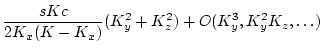
process carry energy between neighboring rays. At first sight, it
would appear that that is indeed the case, that the modified nonlinear
dispersion law is
)
correction to the frequency leads us to ask if that terms could
provide the dispersion required to allow the usual triad resonance
process carry energy between neighboring rays. At first sight, it
would appear that that is indeed the case, that the modified nonlinear
dispersion law is
While this fact is the principal new result of this paper, our approach lays the foundation for a systematic evaluation of the contribution to energy exchange that occurs at higher order. Indeed, we expect that some of the terms found by Benney and Newell [5] involving gradients across resonant manifolds which, in the fully dispersive case, are not relevant because the resonant three wave interaction gives rise to an isotropic distribution, may be more important in this context.
The paper is written as follows. In the next Section, we derive the equation of motion for acoustic waves of small but finite amplitude. A second approach discussed in Subsect. 2B starts from the Hamiltonian formulation of the Euler equations and again makes use of the small amplitude parameter of the problem to simplify the interaction Hamiltonian. As we will see in Subsect. 2C both approaches are equivalent and which approach to use is the question of taste.
Next, in Section 3 we write down the hierarchy of equations for the spectral cumulants and solve them perturbatively. Certain resonances manifest themselves as algebraic and logarithmic time growth in the formal perturbation expansions and mean that these expansions are not uniformly asymptotic in time. The kinetic equation, describing the long time behavior of the zeroth order spectral energy, and the equations describing the long time behavior of the zeroth order higher cumulants are simply conditions that effectively sum the effect of the unbounded growth terms. Under this renormalization, the perturbation series becomes asymptotically uniform. By asymptotically uniform, we mean that the asymptotic expansion for each of the cumulants remains an asymptotic expansion over long times. All unbounded growths are removed. While this procedure in principle requires one to identify and calculate unbounded terms to all orders, in practice one gains a very good approximation by demanding uniform asymptotic behavior only to that order in the coupling coefficient where the unboundedness first appears.
In other words this means that if one finds that if the first two
terms of the asymptotic expansion are
![]() ,
then the effective removal of
,
then the effective removal of ![]() will remove all terms which are
powers of
will remove all terms which are
powers of
![]() in the full expansion. Likewise, it also
assumes that there appear no worse secular terms at a higher order,
such as for example
in the full expansion. Likewise, it also
assumes that there appear no worse secular terms at a higher order,
such as for example
![]() . To achieve uniformity,
one requires an intimate knowledge of how unbounded growth appears.
This sort of perturbative analysis was first done in the thirties by
Dyson. A technical innovation was to use graph notations, called diagrams, for representing lengthy analytical expressions for high
order terms in the perturbation series. It often happens that one can
find the principal subsequence of terms just by looking on the
topological structure of corresponding diagrams. This method of
treating perturbation approaches is called the diagrammatic
technique.
. To achieve uniformity,
one requires an intimate knowledge of how unbounded growth appears.
This sort of perturbative analysis was first done in the thirties by
Dyson. A technical innovation was to use graph notations, called diagrams, for representing lengthy analytical expressions for high
order terms in the perturbation series. It often happens that one can
find the principal subsequence of terms just by looking on the
topological structure of corresponding diagrams. This method of
treating perturbation approaches is called the diagrammatic
technique.
The first variant of diagrammatic technique for non-equilibrium processes was suggested by Wyld[12] in the context of the Naiver Stokes equation for an incompressible fluid. This technique was later generalized by Martin, Siggia and Rose [13], who demonstrated that it may be used to investigate the fluctuation effects in the low-frequency dynamics of any condensed matter system. In fact this technique is also a classical limit of the Keldysh diagrammatic technique [14] which is applicable to any physical system described by interacting Fermi and Bose fields. Zakharov and L'vov [15] extended the Wyld technique to the statistical description of Hamiltonian nonlinear-wave fields, including hydrodynamic turbulence in the Clebsch variables [16]. In section 4, we will use this particular method for treating acoustic turbulence.
Note that in such a formulation, unbounded growths appear as
divergences (or almost divergences) due to the presence of zero
denominators caused by resonances, the very same resonances, in fact,
that give rise to unbounded growth in our more straightforward
perturbation approach. Moreover, diagrammatic techniques are
schematic methods for identifying all problem terms and for adding
them up. If one uses the diagram technique only to the first order at
which the first divergences appear, this is called the one-loop
approximation and is equivalent to identifying the first long time
nonlinear effects. This is exactly analogous to what we will do in
our first approach in this paper although we will also display the
diagram technique. The one loop approximation will give the same long
time behavior of the system for times of ![]() defined earlier.
In Appendix C we analyze two loop diagrams and show that some of them
gives the same order contribution to
defined earlier.
In Appendix C we analyze two loop diagrams and show that some of them
gives the same order contribution to ![]() as two loop diagrams.
Nevertheless one may believe, that even one-loop approximation gives
qualitatively correct description of the dynamics of the system.
as two loop diagrams.
Nevertheless one may believe, that even one-loop approximation gives
qualitatively correct description of the dynamics of the system.
The last Section 5 is devoted to some concluding remarks and the identification of the remaining challenges. We now begin with deriving the basic equations of motion for weak acoustic turbulence.

![$\displaystyle ( \gamma+1)e({\bf k})e( \gamma {\bf k})\Big]
+\int_0^1d k \alpha(1-\alpha)\Big[ e({\alpha} k) e((1-\alpha){\bf k})$](img93.png)
![$\displaystyle {\alpha} e({\bf k})e((1-\alpha){\bf k})
-(1-\alpha)e(k)e({\alpha} {\bf k}) \Big] \Bigg\}$](img94.png)
![$\displaystyle O( \epsilon ^2)\Bigg] +
i \pi ^2 (\mu+1)^2 \epsilon ^2 \Bigg[\int_{\vert{\bf k}\vert
}^{\infty}\beta^2 e(\beta \hat k) d \beta$](img105.png)
![$\displaystyle \frac{1}{\vert{\bf k}\vert}\int_0^{\vert {\bf k}\vert }
\beta^3 e...
...+ \vert k\vert \int_0^{\vert{\bf k}\vert } \beta e(\beta \hat k) d \beta
\Bigg]$](img106.png)