Canonical Equation of Motion

The Hamiltonian equations of motion (2.12) for the complex canonical variables $b\ b^*$ have standard form[1]

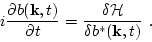$$i{\partial b({\bf k},t)\over\partial t} ={\delta{\cal H}\over\delta b^*({\bf k},t)} \ .$$ (43)

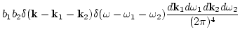
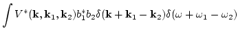
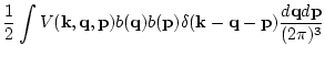
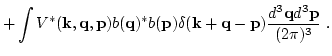
For the acoustic Hamiltonian (2.17-2.19), this equation takes the form

$$\Big[ i \frac{\partial}{\partial t} - c k \Big] b({\bf k},t)$$

$$= \frac{1}{2} \int V({\bf k},{\bf q},{\bf p})b({{\bf q}})b({{\bf p}}) \delta({\bf k}-{\bf q}-{\bf p}) \frac{d {\bf q} d {\bf p}}{(2\pi)^3}$$ (44)

$$+\int V^*({\bf k},{\bf q},{\bf p})b({{\bf q}})^*b({{\bf p}}) \delta({\bf k}+{\bf q}-{\bf p}) \frac{d^3 {\bf q} d^3 {\bf p}}{(2\pi)^3}\ .$$

It is sometimes convenient to concentrate attention on steady state turbulence, which is convenient to describe in the ${\bf k},\omega$ -representation. After performing a time Fourier transform, one has instead of (2.23),

$$\Big[ \omega - c k \Big]b ({\bf k},\omega) = \frac{1}{2} \int V({\bf k},{\bf k}_1,{\bf k}_2)$$

$$\times b_1 b_2 \delta({\bf k}-{\bf k}_1-{\bf k}_2) \delta(\omega-\omega_1-\omega_2) \frac{d {\bf k}_1 d \omega_1 d{\bf k}_2 d\omega _2}{(2\pi)^4}$$

$$+ \int V^*({\bf k},{\bf k}_1,{\bf k}_2)b_1 ^*b_2 \delta({\bf k}+{\bf k}_1-{\bf k}_2) \delta (\omega +\omega_1-\omega_2)$$

$$\times \frac{d {\bf k}_1 d\omega _1 d{\bf k}_2 d\omega _2}{(2\pi)^4} \ .$$ (45)

Hereafter we will refer to this as the basic equation of motion for the acoustic turbulence normal variables $b_k,\ \ b^*_k$ and use it for a statistical description of acoustic turbulence.