Balance Equation

Consider the Dyson-Wyld equations (4.6) and (4.7) in the inertial interval, where one can neglect $\gamma_0({\bf k})$ in comparison with ${\rm Im} \Sigma({\bf k},\omega)$ and $D({\bf k})$ in comparison with $\Phi ({\bf k},\omega )$:

$$G({\bf k},\omega) = \frac{1}{\omega-\omega_0({\bf k}) -\Sigma({\bf k},\omega)} \,,$$ (97)

$$n({\bf k},\omega) = \vert G({\bf k},\omega)\vert^2 \Phi({\bf k},\omega) \ .$$ (98)

It follows from (4.6) that

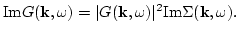$${\rm Im}G({\bf k},\omega)=\vert G({\bf k},\omega)\vert^2{\rm Im} \Sigma({\bf k},\omega).$$ (99)

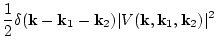
By comparing (4.36) with (4.37) one may see that the following combination

$$L({\bf k},\omega)\equiv \Phi({\bf k},\omega) {\rm Im} G({\bf k},\omega) -n({\bf k},\omega){\rm Im}\Sigma({\bf k},\omega)$$ (100)

is equal to zero. In particular

$$L({\bf k})\equiv\int L({\bf k},\omega) \frac{d\omega}{2\pi}=0\ .$$ (101)

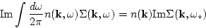
Together with (4.38) it gives

$${\rm Im} \int \frac{d\omega}{2\pi} \left[ \Phi({\bf k},\omeg... ...omega) - n({\bf k},\omega)\Sigma({\bf k},\omega) \right]=0\ .$$ (102)

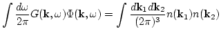
Let us compute now the first term in (4.40). By substitution Eq. (4.34) for $\Phi ({\bf k},\omega )$ and Eq. (4.11) and integration over $\omega$ one has

$$\int \frac{d\omega}{2\pi}G({\bf k},\omega) \Phi({\bf k},\omega)=\int \frac{d{\bf k}_1 d {\bf k}_2}{(2\pi)^3} n({\bf k}_1)n({\bf k}_2)$$

$$\times \Bigg[ \frac{1}{2} \frac{\vert V({\bf k},{\bf k}_1,{\bf k}_2)\ver... ..._2)} {\omega_0({\bf k})-\omega_0({\bf k}_1 )-\omega_0({\bf k}_2)-i\Gamma_{k12}}$$

$$+ \frac{\vert V({\bf k}_2,{\bf k}_1,{\bf k})\vert^2 \delta({\bf k}+... ...a_0({\bf k})+\omega_0({\bf k}_1)-\omega_0({\bf k}_2) -i\Gamma_{k12}} \Bigg] \ .$$ (103)

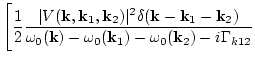
Next we will perform integration over $\omega$ in (4.40). Remember $\Sigma ({\bf k},\omega )$ is analytical function in the upper half plane of $\omega$ while $n({\bf k},\omega)$ has one pole there. Therefore

$${\rm Im} \int \frac{d\omega}{2\pi} n({\bf k}, \omega)\Sigma({\bf k},\omega)= n({\bf k}){\rm Im}\Sigma({\bf k},\omega_*)$$ (104)

where $\omega_*$ is given by (4.15). This is the justification of our choice $\omega_*$.

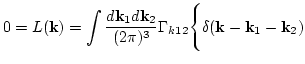
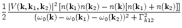
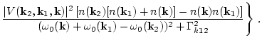
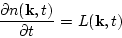
Now let us put everything together to obtain

$$0=L({\bf k})=\int\frac{d{\bf k}_1 d{\bf k}_2}{(2\pi)^3}\Gamma_{k12} \Bigg\{ \delta({\bf k}-{\bf k}_1-{\bf k}_2)$$ (105)

$$\times \frac{1}{2}\frac{\vert V({\bf k},{\bf k}_1,{\bf k}_2)\vert^2 \lef... ...{(\omega_0({\bf k})-\omega_0({\bf k}_1)-\omega_0({\bf k}_2))^2 +\Gamma^2_{k12}}$$

$$+ \delta({\bf k}+{\bf k}_1-{\bf k}_2)$$

$$\times \frac{\vert V({\bf k}_2,{\bf k}_1,{\bf k})\vert^2 \left[n({\bf k}... ...\bf k})+\omega_0({\bf k}_1 )-\omega_0({\bf k}_2))^2+\Gamma^2_{k12}} \Bigg\} \ .$$

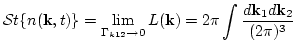
This is the main result of the diagrammatic approach: the balance equation for stationary in time acoustic turbulence. In nonstationary case one can get similarly the generalized kinetic equation in the form

$${\partial n({\bf k}, t)\over \partial t}=L({\bf k}, t)$$ (106)

where $L({\bf k}, t)$ is given by Eq. (4.43) with correlator depending on time $n({\bf k}_j)\to n({\bf k}_j,t)$. In the limit $\gamma ({\bf k}) \to 0$ this expression turns into well known (cf. [1]) collision integral for 3-wave kinetic equation

$${\cal S}t\{n({\bf k}, t) \}=\lim_{\Gamma_{k12}\to 0} L({\bf k}) =2\pi \int\frac{d{\bf k}_1 d{\bf k}_2}{(2\pi)^3}$$

$$\times \frac{1}{2}\delta({\bf k}-{\bf k}_1-{\bf k}_2) \vert V({\bf k},{\bf k}_1,{\bf k}_2)\vert^2$$

$$\left\{n({\bf k}_1)n({\bf k}_2)-n({\bf k})[n({\bf k}_1)+n({\bf k}_2)]\right\}$$

$$\times \delta [\omega_0({\bf k})-\omega_0({\bf k}_1)-\omega_0({\bf k}_2)]$$

$$+ \delta({\bf k}+{\bf k}_1-{\bf k}_2) \vert V({\bf k}_2,{\bf k}_1,{\bf k})\vert^2$$

$$\left\{n({\bf k}_2)[n({\bf k}_1)+n({\bf k})] -n({\bf k})n({\bf k}_1)\right\}$$

$$\times \delta [\omega_0({\bf k})+\omega_0({\bf k}_1)-\omega_0({\bf k}_2)] \ .$$ (107)

We see that the generalized kinetic equation differs from the well known collision term in the three wave kinetic equation by replacing $\delta$-functions on the corresponding Lorenz function with the width of $\Gamma_{k12}$-triad interaction frequency.