Now we can observe that all contributions to the
evolution of ![]() (namely
(namely ![]() , see the previous section and Appendix 2)
contain factor
, see the previous section and Appendix 2)
contain factor
![]() which means that the phase factors
which means that the phase factors ![]() remain a set of statistically independent (of each each other and
of
remain a set of statistically independent (of each each other and
of ![]() 's) variables uniformly distributed on
's) variables uniformly distributed on ![]() . This is true with
accuracy
. This is true with
accuracy
![]() (assuming that the
(assuming that the ![]() -limit is taken first, i.e.
-limit is taken first, i.e.
![]() ) and this proves persistence of the first of the
``essential RPA'' properties. Similar result
for a special class of three-wave systems arising in the solid state physics
was previously obtained by Brout and Prigogine [16].
This result is interesting
because it has been obtained without any assumptions on the
statistics of the amplitudes
) and this proves persistence of the first of the
``essential RPA'' properties. Similar result
for a special class of three-wave systems arising in the solid state physics
was previously obtained by Brout and Prigogine [16].
This result is interesting
because it has been obtained without any assumptions on the
statistics of the amplitudes ![]() and, therefore, it is valid
beyond the RPA approach. It may appear useful in future for study of
fields with random phases but correlated amplitudes.
and, therefore, it is valid
beyond the RPA approach. It may appear useful in future for study of
fields with random phases but correlated amplitudes.
Let us now derive an evolution equation for the generating functional.
Using our results for ![]() in (18) and (17) we have
in (18) and (17) we have
Let us now ![]() limit followed by
limit followed by
![]() (we re-iterate that this order of the limits is essential).
Taking into account that
(we re-iterate that this order of the limits is essential).
Taking into account that
![]() , and
, and
![]() and,
replacing
and,
replacing
![]() by
by ![]() we have
we have
![$\displaystyle {\epsilon}^2
\sum_{j,m,n}(\lambda_{j}+\lambda_{j}^2 {\partial \ov...
...n}^{m}
\right]
{\partial^2 Z(0)\over \partial \lambda_{m} \partial \lambda_{n}}$](img232.png)
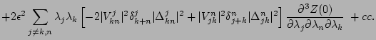
![$\displaystyle + 4{\epsilon}^2 \sum_{j,m,n}
\lambda_j
\left[ - \vert V_{mn}^j\ve...
...partial \lambda_{n}} \right)
\right]
{\partial Z(0) \over \partial \lambda_{j}}$](img233.png)
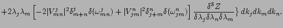
![$\displaystyle 4 \pi {\epsilon}^2
\int \big\{ (\lambda_{j}+\lambda_{j}^2 {\delta...
...delta_{j+n}^{m}
\right]
{\delta^2 Z\over \delta \lambda_{m} \delta \lambda_{n}}$](img243.png)
![$\displaystyle + 2
\lambda_j
\left[ - \vert V_{mn}^j\vert^2 \delta(\omega_{mn}^j...
...a \over \delta \lambda_{n}} \right)
\right]
{\delta Z \over \delta \lambda_{j}}$](img244.png)