


Next: Equation for
Up: Evolution of the multi-mode
Previous: Asymptotic expansion of the
Let us consider the initial fields
 are essentially RPA as defined above. We will perform
averaging over the statistics of the initial fields
in order to obtain an evolution equations, first for
are essentially RPA as defined above. We will perform
averaging over the statistics of the initial fields
in order to obtain an evolution equations, first for  and
then for the multi-mode PDF.
The ultimate goal of this exercise is to prove that
the wavefield remains of the essentially RPA type over the
nonlinear time.
and
then for the multi-mode PDF.
The ultimate goal of this exercise is to prove that
the wavefield remains of the essentially RPA type over the
nonlinear time.
Let us introduce a graphical classification of the above terms which
will allow us to simplify the statistical averaging and to understand
which terms are dominant. We will only consider here contributions from
 and
and  which will allow us to understand the basic method.
Calculation of the rest of the terms,
which will allow us to understand the basic method.
Calculation of the rest of the terms,  ,
,  and
and  ,
follows the same principles and can be found in Appendix 2.
First,
The linear in
,
follows the same principles and can be found in Appendix 2.
First,
The linear in  terms are represented by which, upon using
(9), becomes
terms are represented by which, upon using
(9), becomes
Hereafter we omit, for brevity of notation, the super-script  because no other super-scripts will appear from now on.
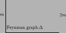
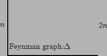
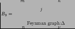
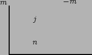
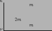
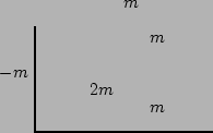
Let us introduce some graphical notations for a simple classification
of different contributions to this and to other (more lengthy)
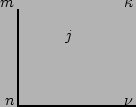
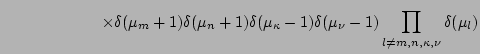
formulae that will follow. Combination
 will
be marked by a vertex joining three lines with in-coming
will
be marked by a vertex joining three lines with in-coming  and
out-coming
and
out-coming  and
and  directions. Complex conjugate
 will be drawn by the same vertex but with the opposite
in-coming and out-coming directions. Presence of
will be drawn by the same vertex but with the opposite
in-coming and out-coming directions. Presence of  and
and  will be indicated by dashed lines pointing away and toward the vertex
respectively. 3 Thus, the two terms in formula (24)
can be schematically represented as follows,
will be indicated by dashed lines pointing away and toward the vertex
respectively. 3 Thus, the two terms in formula (24)
can be schematically represented as follows,
Let us average over all the independent phase factors in the set
 .
Such averaging takes into account the statistical
independence and uniform distribution of
variables
.
Such averaging takes into account the statistical
independence and uniform distribution of
variables  . In particular,
 ,
,
 and
and
 . Further, the products that involve
odd number of 's are always zero, and among the even
products only those can survive that have equal numbers of
's and
. Further, the products that involve
odd number of 's are always zero, and among the even
products only those can survive that have equal numbers of
's and  's. These 's and 's
must cancel each other which is possible if their indices
are matched in a pairwise way similarly to the Wick's
theorem. The difference with the standard Wick, however, is
that there exists possibility of not only internal
(with respect to the sum) matchings but also external
ones with 's in the pre-factor
's. These 's and 's
must cancel each other which is possible if their indices
are matched in a pairwise way similarly to the Wick's
theorem. The difference with the standard Wick, however, is
that there exists possibility of not only internal
(with respect to the sum) matchings but also external
ones with 's in the pre-factor
 .
.
Obviously, non-zero contributions can only arise for terms in which
all 's cancel out either via internal mutual couplings within
the sum or via their external couplings to the 's in the
 -product. The internal couplings will indicate by joining the
dashed lines into loops whereas the external matching will be shown as
a dashed line pinned by a blob at the end. The number of blobs in
a particular graph will be called the valence of this graph.
-product. The internal couplings will indicate by joining the
dashed lines into loops whereas the external matching will be shown as
a dashed line pinned by a blob at the end. The number of blobs in
a particular graph will be called the valence of this graph.
Note that there will be no
contribution from the internal couplings between the incoming and the
out-coming lines of the same vertex because, due to the
 -symbol, one of the wavenumbers is 0 in this case, which means
4that
-symbol, one of the wavenumbers is 0 in this case, which means
4that  . For we have
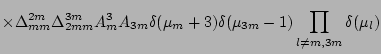
with
and
which correspond to the following expressions,
and
Because of the -symbols involving  's, it takes very
special combinations of the arguments in
's, it takes very
special combinations of the arguments in  for the
terms in the above expressions to be non-zero. For example, a
particular term in the first sum of (25) may be non-zero if
two 's in the set
for the
terms in the above expressions to be non-zero. For example, a
particular term in the first sum of (25) may be non-zero if
two 's in the set  are equal to 1 whereas the rest of
them are 0. But in this case there is only one other term in this sum
(corresponding to the exchange of values of and ) that may be
non-zero too. In fact, only utmost two terms in the both
(25) and (26) can be non-zero simultaneously. In
the other words, each external pinning of the dashed line removes
summation in one index and, since all the indices are pinned in the
above diagrams, we are left with no summation at all in i.e. the
number of terms in is
are equal to 1 whereas the rest of
them are 0. But in this case there is only one other term in this sum
(corresponding to the exchange of values of and ) that may be
non-zero too. In fact, only utmost two terms in the both
(25) and (26) can be non-zero simultaneously. In
the other words, each external pinning of the dashed line removes
summation in one index and, since all the indices are pinned in the
above diagrams, we are left with no summation at all in i.e. the
number of terms in is  with respect to large
  . We will
see later that the dominant contributions have
. We will
see later that the dominant contributions have  terms. Although these terms come in the
  order, they will be
much greater that the
order, they will be
much greater that the  terms because the limit
  must always be taken before
 .
.
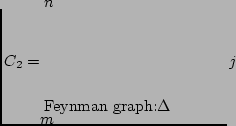
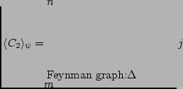
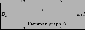
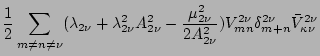
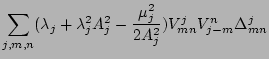
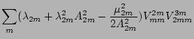
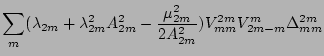
Let us consider the first of the -terms, . Substituting
(9) into (20), we have
where
Here the graphical notation for the interaction coefficients  and
the amplitude
and
the amplitude  is the same as introduced in the previous section and
the dotted line with index indicates that there is a summation over
but there is no amplitude in the corresponding expression.
is the same as introduced in the previous section and
the dotted line with index indicates that there is a summation over
but there is no amplitude in the corresponding expression.
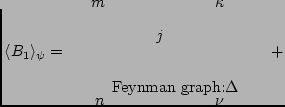
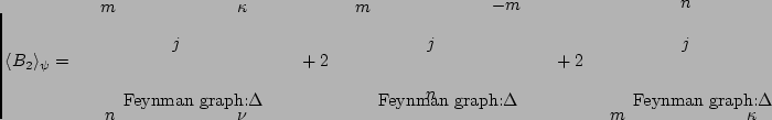
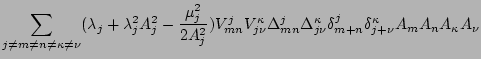
Let us now perform the phase averaging which corresponds to the internal and external
couplings of the dashed lines. For
 we have
 |
|
|
(28) |
where
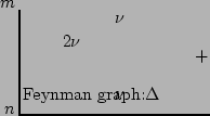
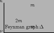
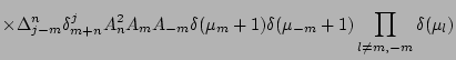
We have not written out the third term in (29) because
it is just a complex conjugate of the second one. Observe that all the
diagrams in the first line of (29) are with
respect to large because all of the summations are lost due to the
external couplings(compare with the previous section). On the other
hand, the diagram in the second line contains two purely-internal
couplings and is therefore . This is because the number of
indices over which the summation survives is equal to the number of
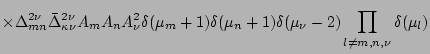
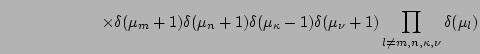
purely internal couplings. Thus, the zero-valent graphs
are dominant and we can write
![$\displaystyle \langle B_1\rangle_\psi = \prod_l\delta(\mu_l)\sum_{j,m,n}(\lambd...
...}^{j}\vert^2
\vert\Delta_{mn}^{j}\vert^2
\delta_{m+n}^{j}A_m^2A_n^2[1+O(1/N^2)]$](img195.png) |
|
|
(29) |
For
 we have
 |
|
|
(30) |
where
The second term in (31) contains one summation because its graph
has one purely internal coupling. This term is times smaller than
the largest terms in
 (which have 2
surviving summation indices). All the other terms in (31)
contain no summation at all because all their dashed lines are coupled
externally.
(which have 2
surviving summation indices). All the other terms in (31)
contain no summation at all because all their dashed lines are coupled
externally.
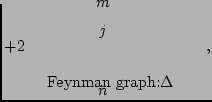
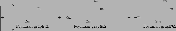
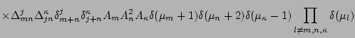
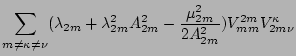
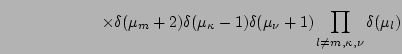
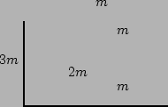
Similarly, the leading contribution to
 will
be given by the zero-valent graph with the maximum possible number of internal
couplings (which is equal to 2 in this case). Because of the
's, there are no graphs with just one internal coupling, but
there are graphs with all the dashed lines coupled externally. Thus,
will
be given by the zero-valent graph with the maximum possible number of internal
couplings (which is equal to 2 in this case). Because of the
's, there are no graphs with just one internal coupling, but
there are graphs with all the dashed lines coupled externally. Thus,
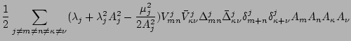
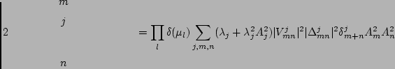
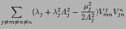
Summarising the results of this section we can write for :
![$\displaystyle J_2 = \prod_{l}\delta(\mu_l)\sum_{j,m,n}(\lambda_{j}+\lambda_{j}^...
... \vert\Delta_{jn}^{m}\vert^2 \delta_{j+n}^{m}
\right]
A_m^2A_n^2 \; [1+O(1/N)].$](img224.png) |
|
|
(32) |
Thus, we considered in detail the different terms involved
in and we found that the dominant contributions come
from the zero-valent graphs because the have more summation
indices involved. This turns out to be the general rule that
allows one to simplify calculation by discarding a significant
number of graphs with non-zero valence.
After this observation finding the rest of the terms,
to , becomes a routine task and we therefore move it to
the Appendix 2.
Next: Equation for
Up: Evolution of the multi-mode
Previous: Asymptotic expansion of the
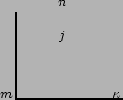
Dr Yuri V Lvov
2007-01-17


![$\displaystyle \parbox{25mm} {
\begin{fmffile}{n19p}
\begin{fmfgraph*}(70,50) \f...
...s_arrow, left=.7, label= $n$}{v2,v1}
\end{fmfgraph*}\end{fmffile}}
[1+O(1/N^2)]$](img222.png)
![$\displaystyle %YL
=2 \prod_{l}\delta(\mu_l)\sum_{j,m,n}(\lambda_{j}+\lambda_{j}...
...vert^2 \vert\Delta_{jn}^{m}\vert^2 \delta_{j+n}^{m}A_m^2A_n^2 \; [1+O(1/N^2)]
,$](img223.png)