Asymptotic expansion of the generating functional.

Let us first obtain an asymptotic weak-nonlinearity expansion for the generating functional $Z\{\lambda, \mu\}$ exploiting the separation of the linear and nonlinear time scales. ² To do this, we have to calculate $Z$ at the intermediate time $t=T$ via substituting into it $a_j(T)$ from (8) and retaining the terms up to $O({\epsilon}^2)$ only. This calculation is given in the Appendix and the result of it is:

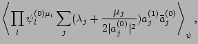
$$Z\{\lambda, \mu, T\} = X\{\lambda, \mu,T\} + \bar X \{\lambda, - \mu,T\}$$ (16)

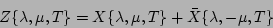
with

$$X\{\lambda, \mu,T\} = X(0) + (2 \pi)^{2N} \left<\prod_{\Vert... ...+{\epsilon}^2(J_2 +J_3+J_4+J_5)] \right>_A + O({\epsilon}^4),$$ (17)

where

$$J_1 = \left<\prod_l \psi_l^{(0)\mu_l} \sum_j (\lambda_j +\frac{\mu_j}{2\vert a_j^{(0)}\vert^2})a_j^{(1)}\bar a_j^{(0)}\right>_\psi,$$ (18)

$$J_2 = {1 \over 2} \left<\prod_l \psi_l^{(0)\mu_l} \sum_j (\lambda_j+ \l... ...^2-\frac{\mu_j^2}{2\vert a_j^{(0)}\vert^2})\vert a_j^{(1)}\vert^2 \right>_\psi,$$ (19)

$$J_3 = \left<\prod_l \psi_l^{(0)\mu_l} \sum_j (\lambda_j + \frac{\mu_j}{2\vert a_j^{(0)}\vert^2})a_j^{(2)}\bar a_j^{(0)} \right>_\psi,$$ (20)

$$J_4 = \left<\prod_l \psi_l^{(0)\mu_l} \sum_j \left[\frac{\lambda_j^2}{2... ...mu_j}{2\vert a_j^{(0)}\vert^2} \right](a_j^{(1)}\bar a_j^{(0)})^2 \right>_\psi,$$ (21)

$$J_5 = {1 \over 2} \left<\prod_l \psi_l^{(0)\mu_l} \sum_{j \ne k}\lambda... ...)}\bar a_k^{(0)} -\bar a_k^{(1)}a_k^{(0)})a_j^{(1)}\bar a_j^{(0)} \right>_\psi,$$ (22)

where $\left< \cdot \right>_A$ and $\left< \cdot \right>_\psi$ denote the averaging over the initial amplitudes and initial phases (which can be done independently). Our next step will be to calculate the above terms by substituting into them the values of $a^{(1)}$ and $a^{(2)}$ from (9) and (10) respectively.