


Next: Statistical description
Up: Noisy spectra, long correlations,
Previous: Random phases vs Gaussian
Consider weakly nonlinear dispersive waves in a periodic box.
Here we consider quadratic nonlinearity and the linear dispersion
relations  which allow three-wave interactions. Example of
such systems include surface capillary waves [4] and
internal waves in the ocean [9]. In Fourier space, the general
form for the Hamiltonian systems with quadratic nonlinearity looks as
follows,
which allow three-wave interactions. Example of
such systems include surface capillary waves [4] and
internal waves in the ocean [9]. In Fourier space, the general
form for the Hamiltonian systems with quadratic nonlinearity looks as
follows,![[*]](file:/usr/share/latex2html/icons/footnote.png)
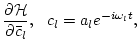
where  is the complex wave amplitude in the interaction representation,
 ,
,  is the box side length,
 for 2D, or
 in 3D, (similar for
  and
and  ),
),
 and
and
 is the wave linear dispersion relation. Here,
 is an interaction coefficient and
  is
introduced as a formal small nonlinearity parameter.
is
introduced as a formal small nonlinearity parameter.
In order to filter out fast oscillations at the wave period, let us
seek for the solution at time  such that
 . The second condition ensures that is a lot
less than the nonlinear evolution time. Now let us use a perturbation
expansion in small ,
. The second condition ensures that is a lot
less than the nonlinear evolution time. Now let us use a perturbation
expansion in small ,
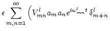
Substituting this expansion in (2) we get in
the zeroth order
 ,
i.e. the zeroth order term is time independent. This corresponds to
the fact that the interaction representation wave amplitudes are
constant in the linear approximation. For simplicity, we will write
,
i.e. the zeroth order term is time independent. This corresponds to
the fact that the interaction representation wave amplitudes are
constant in the linear approximation. For simplicity, we will write
 , understanding that a quantity is taken at
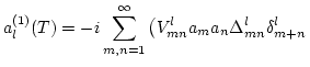
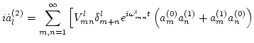
  if its time argument is not mentioned explicitly. The first order is
given by
if its time argument is not mentioned explicitly. The first order is
given by
 |
|
|
|
 |
|
|
(3) |
where
 Here we have taken into account that
 and
and
 .
.
To calculate the second iterate, write
We now have to substitute (3) into
(4) and integrate over time to obtain
-------------------------------------
-----------------------------------
--
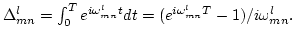
where we used
 and introduced
Next: Statistical description
Up: Noisy spectra, long correlations,
Previous: Random phases vs Gaussian
Dr Yuri V Lvov
2007-04-11
![$\displaystyle \sum_{m,n, \mu, \nu=1}^\infty \left[ 2 V^l_{mn}
\left(
-V^m_{\mu ...
...l \nu}_{n \mu},\omega^l_{mn}]\delta^\mu_{m + \nu}\right)
\delta^l_{m+n} \right.$](img69.png)