Random phases vs Gaussian fields --

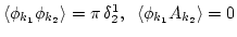
The random phase approximation (RPA) has been popular in WT because it allows a quick derivation of KE [1,3]. We will use RPA in this paper because it provides a minimal model for for description of the k-space fluctuations of the waveaction about its mean spectrum, but we will also discuss relation to the approach of [2] which does not assume RPA. By definition, RPA for an ensemble of complex fields $a_k = A_k e^{i\phi_k}$ means that the phases $\phi_k$ are uniformly distributed in $(0,2\pi]$ and are statistically independent of each other and of the amplitude $A_k$, $\langle \phi_{k_1} \phi_{k_2} \rangle = \pi \delta^1_2, \;\; \langle \phi_{k_1} A_{k_2} \rangle = 0$. Thus, the averaging over the phase and over the amplitude statistics can be performed independently. In RPA, the fluctuations of the amplitudes $A_k$ must also be decorrelated at different $k$'s, $\langle A_{k_1}^n A_{k_2}^m \rangle =\langle A_{k_1}^n \rangle \langle A_{k_2}^m \rangle \;\; (m,n = 1,2,3,...)$.

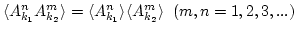To illustrate the relation between the random phases and Gaussianity, let us consider the fourth-order moment for which RPA gives

$$\langle a_{k_1} a_{k_2} {\overline a_{k_3}} {\overline a_{k_... ...lta^2_3) + Q_{k_1} \delta^1_{2} \delta^{1}_{3} \delta^{1}_{4},$$ (1)

where $n_k = \langle A_{k}^2 \rangle$ is the waveaction spectrum and $Q_k = \langle A_{k}^4 \rangle$ is a cumulants coefficient. The last term in this expression appears because the phases drop out for $k_1=k_2=k_3=k_4$ and their statistics poses no restriction on the value of this correlator at this point. This cumulant part of the correlator can be arbitrary for a general random-phased field whereas for Gaussian fields $Q_k$ must be zero. Such a difference between the Gaussian and the random-phased fields occurs only at a vanishingly small set of modes with $k_1=k_2=k_3=k_4$ and it has been typically ignored before because its contribution to KE is negligible. 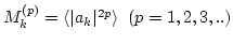Therefore, if the mean waveaction spectrum was the only thing we were interested in, we could safely ignore contributions from all (one-point) moments $M^{(p)}_k = \langle \vert a_{k}\vert^{2p} \rangle \;\; (p=1,2,3,..)$.

However, it is precisely moments $M^{(p)}_k$ that contain information about fluctuations of the waveaction about its mean spectrum. For example, the standard deviation of the waveaction from its mean is $\sigma_k = (\langle \vert a_{k}\vert^4 \rangle - \langle \vert a_{k}\vert^2 \rangle^2)^{1/2} = (M^{(2)}_k - n_k^2)^{1/2}$. This quantity can be arbitrary for a general random-phased field whereas for a Gaussian wave field the fluctuation level $\sigma_k$ is fixed, $\sigma_k = n_k$. Note that different values of moments $M^{(p)}_k$ can correspond to hugely different typical wave field realizations. In particular, if $M^{(p)} = n^p$ then there is no fluctuations and $A_k$ is deterministic, $\sigma_k=0$. For the opposite extreme of large fluctuations we would have $M^{(p)} \gg n^p$ which means that the typical realization is sparse in the k-space and is characterized by few intermittent peaks of $A_k$ and close to zero values in between these peaks. Note that the information about the spectral fluctuations of the waveaction contained in the one-point moments $M^{(p)}$ is completely erased from the multiple-point moments by the random phases and it is precisely why these new objects play a crucial role for the description of the fluctuations.

Will the waveaction fluctuations appear if they were absent initially? Will they saturate at the Gaussian level $\sigma_k = n_k$ or will they keep growing leading to the k-space intermittency? To answer these questions, we will use RPA to derive and analyze equations for the moments $M^{(p)}_k$ for arbitrary orders $p$ and thereby describe the statistical evolution of the spectral fluctuations. Note that RPA, without a stronger Gaussianity assumption, is totally sufficient for the WT closure at any order. This allows us to study wavefields with moments $M^{(p)}_k$ very far from their Gaussian values, which may happen, for example, because of the choice of initial conditions or a non-Gaussianity of the energy source in the system.

In [2] non-Gaussian fields of a rather different kind were considered. Namely, statistically homogeneous wave fields were considered in an infinite space which initially have decaying correlations in the coordinate space and, therefore, smooth cumulants in the k-space, e.g.

$$\langle a_{k_1} a_{k_2} {\overline a_{k_3}} {\overline a_{k_... ...{k_1}_{k_4}\delta^2_3) + C_{123} \delta^{k_1+k_2}_{k_3 + k_4},$$

where $C_{123}$ is a smooth function of $k_1, k_2, k_3$ and $\delta$'s now mean Dirac deltas. On the other hand, by taking the large box limit it is easy to see that our expression (1) corresponds to a singular cumulant $C_{123} = Q_{k_1}/{\cal V} \delta^{k_1}_{k_2} \delta^{k_1}_{k_3}$. It tends to zero when the box volume ${\cal V}$ tends to infinity and yet it gives a finite contribution to the waveaction fluctuations in this limit.This singular cumulant corresponds to a small component of the wavefield which is long-correlated - the case not covered by the approach of [2]. On the other hand, it would be straightforward to go beyond our RPA by adding a cumulant part of the initial fields which tends to a smooth function of $k_1, k_2, k_3$ in the infinite box limit (like in [2]). However, such cumulants would give a box-size dependent contribution to the waveaction fluctuations which vanishes in the infinite box limit (e.g. it would change $\sigma_k^2$ by $C_{kkk}/{\cal V}$). Thus, in large boxes the waveaction fluctuation for the fields with smooth cumulants is fixed at the same value as the for Gaussian fields, $\sigma_k = n_k$, and introduction of the singular cumulant is essential to remove this restriction on the level of fluctuations. On the other hand, the smooth part of the cumulants has no bearing on the closure, as shown in [2] and on the large-box fluctuation and, therefore, will be omitted here for brevity and clarity of the analysis.