... $\langle \phi_{k_1} \phi_{k_2} \rangle = \pi \delta^1_2, \;\; \langle \phi_{k_1} A_{k_2} \rangle = 0$

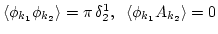
We start by considering fields in a periodic box which is an essential intermediate step in the definition of RPA and the new correlators $M^{(p)}_k$ introduced later in this work. Therefore $\delta^1_2$ here is the Kronecker symbol. Later, we take the large box limit corresponding to homogeneous wave turbulence.

.
.
.
.
.
.
.
.
.
.
.
.
.
.
.
.
.
.
.
.
.
.
.
.
.
.
.
.
.
.

...'s

This property is typically not mentioned explicitly (but used implicitly) when RPA is employed.

.
.
.
.
.
.
.
.
.
.
.
.
.
.
.
.
.
.
.
.
.
.
.
.
.
.
.
.
.
.

... limit.

Thus, assuming a finite box is an important intermediate step when introducing the relevant to the fluctuations objects like $Q_k$.

.
.
.
.
.
.
.
.
.
.
.
.
.
.
.
.
.
.
.
.
.
.
.
.
.
.
.
.
.
.

... follows,

We will follow the RPA approach as presented by Galeev and Sagdeev [3] but deal with a slightly more general case where the wave field is not restricted by the condition $\overline a(k) = a(-k)$. We will also use elements of the technique and notations of [2].

.
.
.
.
.
.
.
.
.
.
.
.
.
.
.
.
.
.
.
.
.
.
.
.
.
.
.
.
.
.

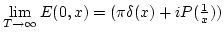
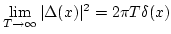
... limit

The large box limit implies that sums will be replaced with integrals, the Kronecker deltas will be replaced with Dirac's deltas, $\delta^l_{m+n}\to\delta^l_{mn}/{\cal V}$, where we introduced short-hand notation, $\delta^l_{mn}=\delta(k_l-k_m-k_n)$. Further we redefine $M^{(p)}_k/{\cal V}^p \to M^{(p)}_k$.

.
.
.
.
.
.
.
.
.
.
.
.
.
.
.
.
.
.
.
.
.
.
.
.
.
.
.
.
.
.

...)

Note that $\lim\limits_{T\to\infty}E(0,x)= (\pi \delta(x)+iP(\frac{1}{x}))$, and $\lim\limits_{T\to\infty}\vert\Delta(x)\vert^2=2\pi T\delta(x)$ (see e.g. [2]).

.
.
.
.
.
.
.
.
.
.
.
.
.
.
.
.
.
.
.
.
.
.
.
.
.
.
.
.
.
.