Next: Discussion
Up: Noisy spectra, long correlations,
Previous: Time-scale separation analysis
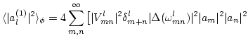
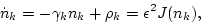
Let us now develop a statistical
description applying RPA to the fields  . Since phases and
the amplitudes are statistically independent in RPA, we will first
average over the random phases (denoted as
. Since phases and
the amplitudes are statistically independent in RPA, we will first
average over the random phases (denoted as
 ) and then we average over amplitudes (denoted as
 ) to calculate the moments,
First, let us calculate
 as
as
-------------------------------------
-----------------------------------
--
where  is the binomial coefficient.
Up to the second power in  terms, we have
Here, the terms
proportional to dropped out after the phase averaging.
Further, we assume that there is no coupling to the  mode, i.e.
 , so that there is no
contribution of the
term like
, so that there is no
contribution of the
term like
 .
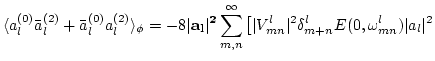
We now use (3) and (5)
and the averaging over the phases to obtain
.
We now use (3) and (5)
and the averaging over the phases to obtain
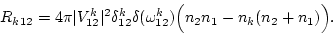
Let us substitute these expressions into (6), perform
amplitude averaging, take the large box limit![[*]](file:/usr/share/latex2html/icons/footnote.png) and then large
and then large  limit (
 ). We have
 |
(4) |
with
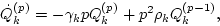
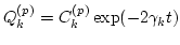
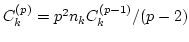
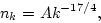
Now, assuming that is a lot less than the nonlinear time (
 ) we finally arrive at our main result,
 |
(7) |
In particular, for the waveaction spectrum  (10) gives the familiar kinetic equation (KE)
 |
(8) |
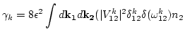
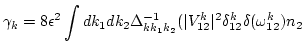
where  is the ``collision'' term [1,3],
with
 |
(9) |
The second equation in the series (10) allows to
obtain the r.m.s.
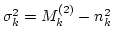 of the fluctuations
of the waveaction
of the fluctuations
of the waveaction
 . We emphasize that
(10) is valid even for strongly intermittent fields
with big fluctuations.
. We emphasize that
(10) is valid even for strongly intermittent fields
with big fluctuations.
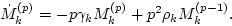
Let us now consider the stationary solution of (10),
 for all
  . Then for
  from (11) we
have
from (11) we
have
 . Substituting this into
(10) we have
. Substituting this into
(10) we have
with the solution
 .
Such a set of moments correspond to a Gaussian wavefield
.
Such a set of moments correspond to a Gaussian wavefield  . To
see how such a Gaussian steady state forms in time, let us rewrite
(10) in terms of the deviations of
. To
see how such a Gaussian steady state forms in time, let us rewrite
(10) in terms of the deviations of  from
their Gaussian values,
from
their Gaussian values,
 Then use (10) to obtain
 |
(10) |
for  This results has a particularly simple form for
  ,
because
,
because
 and we get a decoupled equation
According to this equation the
deviations from Gaussianity can grow or decay depending on the sign of
 . However, according to KE near the steady state
 (because
  is always positive), the deviations from
Gaussianity decay. A similar picture arises also for the higher
moments. The easiest way to see this is to choose initial conditions
where
is always positive), the deviations from
Gaussianity decay. A similar picture arises also for the higher
moments. The easiest way to see this is to choose initial conditions
where  is already at its steady value (but not the higher
moments). Then (13) becomes a linear system which can
be immediately solved as an eigenvalue problem. For large time, the
largest of these eigenvalues,
is already at its steady value (but not the higher
moments). Then (13) becomes a linear system which can
be immediately solved as an eigenvalue problem. For large time, the
largest of these eigenvalues,
 , will dominate
and the solutions tend to
, will dominate
and the solutions tend to
 where
where  satisfy a recursive relation
 and
and  is arbitrary (determined by the
initial conditions). Thus we conclude that the steady state
corresponding to a Gaussian wavefield is stable.
is arbitrary (determined by the
initial conditions). Thus we conclude that the steady state
corresponding to a Gaussian wavefield is stable.
Predictions of equation (10) about the behavior of
fluctuations of the waveaction spectra can be tested by modern
experimental techniques which allow to produce surface water waves
with random phases and a prescribed shape of the amplitude  [11]. It is even easier to test (10)
numerically. Consider for example capillary waves on deep water. If
a Gaussian forcing at low
[11]. It is even easier to test (10)
numerically. Consider for example capillary waves on deep water. If
a Gaussian forcing at low  values is present, the steady state
solution of the kinetic equation corresponds to the Zakharov-Filonenko
(ZF) spectrum of Kolmogorov type [1,4]. It is given by
values is present, the steady state
solution of the kinetic equation corresponds to the Zakharov-Filonenko
(ZF) spectrum of Kolmogorov type [1,4]. It is given by
 |
(11) |
with
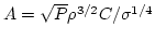 , where
  is the value of flux of energy toward high wavenumbers, and
 are the density and surface tension of water, and
  . The simplest experiment would be to start with a
zero-fluctuation (deterministic) spectrum and to compare the
fluctuation growth with the predictions of (10).
Note that such no-fluctuations initial conditions were used in
[6,7].
. The simplest experiment would be to start with a
zero-fluctuation (deterministic) spectrum and to compare the
fluctuation growth with the predictions of (10).
Note that such no-fluctuations initial conditions were used in
[6,7].
Let us calculate the rate at which a fluctuations grow for such an
initial conditions. To do that let us assume that the spectrum  is isotropic, that is it depends only on the modulus of the vector,
not on its directions. We then can make an angular averaging of
(9) obtaining:
is isotropic, that is it depends only on the modulus of the vector,
not on its directions. We then can make an angular averaging of
(9) obtaining:
Let us substitute ZF spectrum (14) into
(![[*]](file:/usr/share/latex2html/icons/crossref.png) ), take the values of
), take the values of  and
and
 appropriate for the capillary waves on deep
water([1], eqs (5.2.1-2)). By changing the variables of
integrations via
appropriate for the capillary waves on deep
water([1], eqs (5.2.1-2)). By changing the variables of
integrations via
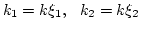 we can factor out
the dependence of
we can factor out
the dependence of  . Performing one of
  integrals
analytically with the use of the delta function in
integrals
analytically with the use of the delta function in  's, we
perform the remaining single integral numerically to obtain (all the
integrals converge):
's, we
perform the remaining single integral numerically to obtain (all the
integrals converge):
where the dimensionless constant  was obtained by numerical
integration. Consequently, our prediction for the fluctuations growth
is
was obtained by numerical
integration. Consequently, our prediction for the fluctuations growth
is
 |
|
|
|
 |
|
|
(12) |
etc. Note that fluctuations stabilize at Gaussian values faster for
high values. It is also interesting to test equation
(10) when the forcing (and therefore the turbulence)
is non-Gaussian, as in most practical situations.
Next: Discussion
Up: Noisy spectra, long correlations,
Previous: Time-scale separation analysis
Dr Yuri V Lvov
2007-04-11