Next: Bibliography
Up: text
Previous: The order -
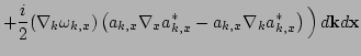
Let us start with the GP equation written in the Hamiltonian form:
 |
(63) |
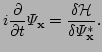
The Hamiltonian for the GP equation (![[*]](file:/usr/share/latex2html/icons/crossref.png) ) coincides with the
total energy of the system:
) coincides with the
total energy of the system:
 |
(64) |
Let us first consider the case without a condensate. Applying the
Gabor transformation to () we get
 |
(65) |
But if we notice that
we obtain
 |
(66) |
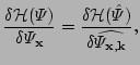
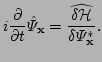
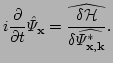
Thus, the time evolution of the Gabor transformed quantity is governed
by the Gabor transformed Hamiltonian equation. However, we would like
to obtain the equation of motion in Hamiltonian form without the Gabor
transformation. Let us re-write () in terms of the
slow amplitudes  defined in ()
 |
(67) |
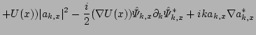
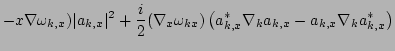
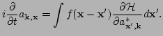
Now, let us express the Hamiltonian
() in terms of the slow variables
,
Here we have integrated by parts
 and, while
calculating the Laplacian of
and, while
calculating the Laplacian of  in terms of slow variables, have
kept only the first order gradients in
in terms of slow variables, have
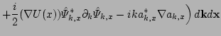
kept only the first order gradients in  . Substituting
() into () allows us to re-write this
equation as
. Substituting
() into () allows us to re-write this
equation as
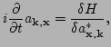 |
(68) |
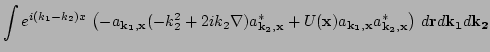
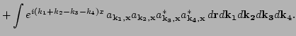
where the filtered Hamiltonian  can be
represented as
can be
represented as
and
 is the Fourier transform of the
  .
.
Expanding  as
as
 and taking into account that
 can be interpreted as
 ,
we have
,
we have
Since
 we can represent the above
formula as
we can represent the above
formula as
Now, we will show that if a condensate is present then the quadratic
part of the Hamiltonian can also be written in the same canonical form
as in (). Let us start from the equation ()
for 
 |
(71) |
with
Expression () for the waveaction in this case allows us to guess the
form of the normal variable,
Note that this expression is consistent with the waveaction considered
above for the case with no condensate. This can be checked by taking
the limit
 . In terms of normal variable
 equations () and () acquire the following
form:
equations () and () acquire the following
form:
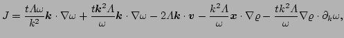
This equation can be represented in the form of a Hamiltonian equation
of motion with a quadratic Hamiltonian as in () when
the frequency is replaced by its Doppler shifted value,
Note that the Doppler
shift does not enter into the equation for the waveaction because it
leads to terms that are of second order in  and therefore
should be neglected.
and therefore
should be neglected.
Next: Bibliography
Up: text
Previous: The order -
Dr Yuri V Lvov
2007-01-23