The $\epsilon^1$ order -

Let us split the wave amplitudes into fastly and slowly varying parts,

$$\lambda(\vec{x},\vec{k},t) = \Lambda(\vec{x},\vec{k},t)\E^{i \vec{k}\cdot\vec{x}+i \omega t}, \mu (\vec{x},\vec{k},t) = M(\vec{x},\vec{k},t)\E^{i \vec{k}\cdot\vec{x}-i \omega t},$$ (47)

or, in shorthand notation,

$$\lambda = \Lambda\E^{+}, \mu = M\E^{-},$$ (48)

where

$$\E^{+} \equiv \E^{i \vec{k}\cdot\vec{x}+i \omega t}, \E^{-} \equiv \E^{i \vec{k}\cdot\vec{x}-i \omega t}.$$

The $\E^{+}$ and $\E^{-}$ represent the fastly oscillating parts of the Gabor transforms. From () it follows that

$$\Lambda^*(\vec{x},-\vec{k},t) = M(\vec{x},\vec{k},t).$$ (49)

Obviously,

$$\partial_{t}\lambda = i \omega\lambda + \E^{+}\partial_{t}\Lambda, \partial_{t}\mu = -i \omega\mu + \E^{-}\partial_{t}M,$$ (50)

$$\nabla\lambda = i \vec{k}\lambda + \E^{+}\nabla\Lambda + i t\lambda\nabla\omega, \nabla\mu = i \vec{k}\mu + \E^{-}\nabla M -i t\mu\nabla\omega,$$ (51)

$$\triangle \lambda = -k^{2}\lambda + 2i \E^{+}\vec{k}\cdot\nabla\Lambda + \E^{+}\triangle\Lambda - 2t\lambda\vec{k}\cdot\nabla\omega,$$ (52)

$$\triangle \mu = -k^{2}\mu + 2i \E^{+}\vec{k}\cdot\nabla M + \E^{+}\triangle M + 2t\mu\vec{k}\cdot\nabla\omega,$$

$$\partial_{k}\lambda = \E^{+}\partial_{k}\Lambda + i \vec{x}\E^{+}\Lambda + i t\E^{+}\Lambda\partial_{k}\omega,$$ (53)

$$\partial_{k}\mu = \E^{-}\partial_{k}M + i \vec{x}\E^{-}M - i t\E^{-}M\partial_{k}\omega.$$

Our aim now is to derive equations for $\partial_{t}\lambda$ and $\partial_{t}\mu$. However, due to the relationship () it is sufficient to derive an equation for only one of the two, for example $\lambda$. From () we find

$$\partial_{t}\lambda = \partial_{t}\left(\frac{\hat{a}}{2} - \frac{i k^{2}}{2\omega}\hat{b}\right).$$

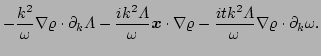
After substituting our equations for $\partial_{t}\hat{a}$ and $\partial_{t}\hat{b}$, () and (), and making use of the relationships () the equation for $\lambda$ acquires the following form:

$$\partial_{t}\lambda = \lambda \left[-\frac{i \nabla\varrho\cdot\nabla\omega}{2k^{2}\v... ...k^{2}\varrho} - 2\vec{v} - \frac{i k^{2}\nabla\varrho}{2\omega\varrho}\right]$$

$$+ \triangle\lambda \left[-\frac{i \omega}{2k^{2}} -\frac{i k^{2}}{2\omega}\right] -\frac{k^{2}}{\omega} \nabla\varrho\cdot\partial_{k}\lambda$$

$$+ \mu \left[\frac{i \nabla\varrho\cdot\nabla\omega}{2k^{2}\varrho... ...la\varrho}{2k^{2}\varrho} - \frac{i k^{2}\nabla\varrho}{2\omega\varrho}\right]$$

$$+ \triangle\mu \left[+\frac{i \omega}{2k^{2}} -\frac{i k^{2}}{2\... ...a}\right] -\frac{k^{2}}{\omega}\nabla\varrho\cdot\partial_{k}\mu - {\cal{NL}}.$$

Here the nonlinear term ${\cal{NL}}$ is given by

$${\cal{NL}}={\cal G} \left[\rho(2 a b + b(a^2+b^2))\right] -\frac{i k^2}{2\omega_k} {\cal G}\left[( \varrho(3 a^2+b^2+a(a^2+b^2)))\right].$$

Note that we have neglected $\dot \omega$ in the above expressions because, according to the dispersion relationship (), it is of the order of $\dot \rho$ which is $O(\epsilon^2)$ by virtue of (). We will also drop the nonlinear term in the subsequent calculation.

Our next step is to eliminate the fast oscillations associated with the Gabor transforms and derive an equation for $\vert\Lambda\vert^{2}$. This in turn will lead to a natural waveaction quantity which can be used to describe the behavior of our wavepackets in phase space. Using (-) we obtain

$$\partial_{t}\Lambda = \Lambda \left[-\frac{i \nabla\varrho\cdot\nabla\omega}{2k^{2}\varrho} + \frac{i k^{2}\varrho}{\omega} -i \omega \right]$$

$$+ \left[i \vec{k}\Lambda+\nabla\Lambda+i t\Lambda\nabla\omega\rig... ...k^{2}\varrho} - 2\vec{v} - \frac{i k^{2}\nabla\varrho}{2\omega\varrho}\right]$$

$$+ \left[-k^{2}\Lambda+2i \vec{k}\cdot\nabla\Lambda-2t\Lambda\vec{... ...ega\right] \left[-\frac{i \omega}{2k^{2}}-\frac{i \vec{k}^{2}}{2\omega}\right]$$

$$-\frac{k^{2}}{\omega}\nabla\varrho\cdot\partial_{k}\Lambda -\fra... ...varrho -\frac{i tk^{2}\Lambda}{\omega}\nabla \varrho \cdot\partial_{k}\omega.$$ (54)

Please note that all the terms involving $M$ drop out. This stems from the fact that, in deriving an equation for $\Lambda$, we have had to divide through by $\E^{+}$. Therefore, any terms involving $M$ will result in a factor

$$\E^{-}/\E^{+} = \E^{-2i \omega t}.$$

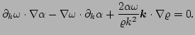
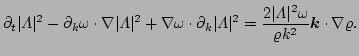
Thus, after time averaging over a few wave periods, all the $M$ terms drop out.

Expanding out equation () we find the $O(1)$ terms cancel out and using the dispersion relationship () we find

$$\partial_{t}\Lambda = \partial_{k}\omega\cdot\nabla\Lambda + \fr... ...k^{2}}\vec{k}\cdot\nabla\varrho - \nabla\omega\cdot\partial_{k}\Lambda + i J ,$$ (55)

where

$$J = \frac{t\Lambda\omega}{k^{2}}\vec{k}\cdot\nabla\omega + \frac... ...bla\varrho - \frac{tk^{2}\Lambda}{\omega}\nabla\varrho\cdot\partial_{k}\omega,$$

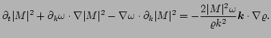
At this point let us drop the nonlinear term and concentrate on the linear dynamics. Multiplying () by $\Lambda^{*}$ and combining it with the complex conjugate equation the $J$ terms cancel, leading to

$$\partial_{t}\vert\Lambda\vert^{2} - \partial_{k}\omega\cdot\nabla... ... \frac{2\vert\Lambda\vert^{2}\omega} {\varrho k^{2}}\vec{k}\cdot\nabla\varrho.$$ (56)

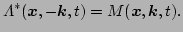
A similar equation for $\vert M\vert^{2}$ can be easily obtained by replacing ${\bf k} \to {- \bf k}$ in () and using (),

$$\partial_{t}\vert M\vert^{2} + \partial_{k}\omega\cdot\nabla\vert... ... = - \frac{2\vert M\vert^{2}\omega} {\varrho k^{2}}\vec{k}\cdot\nabla\varrho.$$ (57)

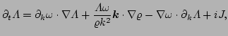
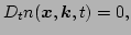
The LHS of this equation is the full time derivative of $\vert M\vert^{2}$ along trajectories. If $\vert M\vert^{2}$ were to be a correct phase-space waveaction, the right hand side of this equation would be zero, however, this is not the case. We find the correct waveaction $n(\vec{x},\vec{k},t)$ by setting

$$\vert M\vert^{2} = \alpha(\vec{x},\vec{k})n(\vec{x},\vec{k},t),$$

and finding such $\alpha(\vec{x},\vec{k})$ that the the full time derivative of $n(\vec{x},\vec{k},t)$ is zero. This leads to the following condition on $\alpha$,

$$\partial_{k}\omega\cdot\nabla\alpha - \nabla\omega\cdot\partial_{k}\alpha + \frac{2\alpha\omega}{\varrho k^{2}}\vec{k}\cdot\nabla\varrho = 0.$$

By choosing $\alpha = k^{X}\varrho^{Y}$ and substituting it to () we find $x=2$, $y=-1$. Therefore the correct form of the waveaction is $n = \frac{\varrho}{k^{2}}\vert M\vert^{2}.$ Summarizing, we have got the following transport equation for the waveaction $n$ in the linear approximation,

$$D_{t}n(\vec{x},\vec{k},t) = 0,$$ (58)

where

$$D_{t}\equiv \partial_{t} + \dot{\vec{x}}\cdot\nabla +\dot{\vec{k}}\cdot\partial_{k},$$ (59)

is the full time derivative along trajectories and

$$\dot{\vec{x}} = \partial_{k} \omega, \hspace{1cm} \dot{\vec{k}} = -\nabla \omega,$$ (60)

are the ray equations with

$$\omega = k \sqrt{k^{2}+2\varrho}.$$ (61)

Obviously, the dynamics in this case cannot be reduced to the Ehrenfest theorem with any shape of potential $U$. Therefore, approaches that model the condensate effect by introducing a renormalized potential are misleading.

Finally, it is useful to express the waveaction $n$ in terms of the original variables,

$$n({\bf k},x,t) = \frac{1}{2} \frac{\omega\rho}{k^{2}} \left\vert... ...hat{ \Re \phi} - \frac{ i k^{2} }{\omega} \widehat{ \Im \phi} \right\vert^{2}.$$ (62)

It is interesting that such a waveaction is in agreement with that found in [13]. In fact in [13] the homogeneous case with non-zero nonlinearity ( $\varepsilon = 0$, $\sigma \neq 0$) was considered. This is the opposite limit to the one we have considered above (where $\varepsilon \neq 0$, $\sigma = 0$).