Next: Weak turbulence for inhomogeneous
Up: text
Previous: Unified WKB description
The derivation for the description of the nonuniform turbulence found
in a BEC system consists of a amalgamation of a WKB method, for the
description of the linear dynamics, and a standard weak turbulence
theory (see e.g. [13]), with the noted modification that
Gabor transforms are used instead of Fourier ones. We will now
demonstrate the general ideas of such a derivation for the simple case
of system where no condensate is present.
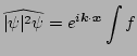
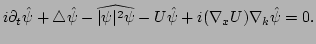
Consider the Gabor transformation of (![[*]](file:/usr/share/latex2html/icons/crossref.png) ):
):
 |
(22) |
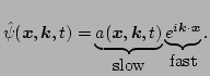
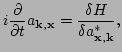
To calculate the
 term let us first separate
the Gabor transform into its correspondingly fast and slow spatial
parts,
term let us first separate
the Gabor transform into its correspondingly fast and slow spatial
parts,
 |
(23) |
Now by using the inverse Gabor transform
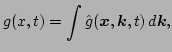 |
(24) |
we find
Note that the slow amplitudes  do not change much over the
characteristic width of the function
do not change much over the
characteristic width of the function  and hence their argument
 can be replaced by
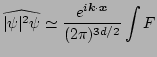
  . Therefore, we can
approximate () by
. Therefore, we can
approximate () by
Here  is the Fourier transform of
  . Note that for the
spatially homogeneous systems,
. Note that for the
spatially homogeneous systems,
 , is just a
delta function,
After dropping terms proportional to
, is just a
delta function,
After dropping terms proportional to
 , equation
() then becomes
, equation
() then becomes
This is the master equation formulating the nonlinear dynamics in
terms of the Gabor amplitudes. This can serve as a starting point for
the statistical averaging which in turn leads to the weak turbulence
formalism. Note that this equation can be written in Hamiltonian form,
 |
(28) |
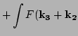
with a Hamiltonian function
where
 . In fact, such a Hamiltonian
description can be derived directly, in terms of the Gabor amplitudes,
from the Hamiltonian formulation of the original GP equation (see
Appendix B).
. In fact, such a Hamiltonian
description can be derived directly, in terms of the Gabor amplitudes,
from the Hamiltonian formulation of the original GP equation (see
Appendix B).
If a condensate is present in the system, one can also re-write the
equations in a Hamiltonian form with an identical quadratic part. That
is, with being replaced by the normal amplitude, and  by
the frequency of waves, found in the presence of the condensate. It
appears that the quadratic part of the Hamiltonian () is
generic in the WKB context. Indeed, let us consider a typical
Hamiltonian for linear waves in weakly inhomogeneous media
[32] expressed in terms of Fourier amplitudes
by
the frequency of waves, found in the presence of the condensate. It
appears that the quadratic part of the Hamiltonian () is
generic in the WKB context. Indeed, let us consider a typical
Hamiltonian for linear waves in weakly inhomogeneous media
[32] expressed in terms of Fourier amplitudes
 and
and

 |
|
|
(30) |
with a hermitian kernel
 which is strongly peaked at
 . As
we will show in a separate paper [26], this Hamiltonian can
be represented in terms of the Gabor transforms as
. As
we will show in a separate paper [26], this Hamiltonian can
be represented in terms of the Gabor transforms as
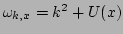
where  are the Gabor coefficients, and
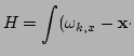
 is
the position dependent frequency, related to
is
the position dependent frequency, related to
 via
via
 |
|
|
(32) |
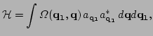
Actually, such an expression is a canonical form, even for a much
broader class of Hamiltonians that correspond to a significant class
of linear equations with coordinate dependent coefficients
[26]. That is,
![$\displaystyle {\cal H}=\int [A({\bf q_1}, {\bf q}) \, a_{\bf q_1} a^*_{\bf q}
\...
...\bf q_1}, {\bf q}) \, a_{\bf q_1} a_{\bf - q} + c.c.] \, d
{\bf q} d {\bf q_1},$](img143.png) |
|
|
(33) |
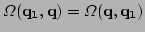
where functions  and
and  peaked at
.
peaked at
.
Next: Weak turbulence for inhomogeneous
Up: text
Previous: Unified WKB description
Dr Yuri V Lvov
2007-01-23