


Next: One-mode statistics
Up: Setting the stage II:
Previous: Wavefields with long spatial
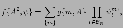
Introduction of generating functionals simplifies statistical
derivations. It can be defined in several different ways
to suit a particular
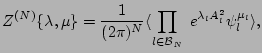
technique. For our problem, the most useful form of the generating
functional is
 |
|
|
(20) |
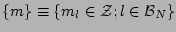
where
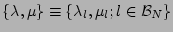 is a set of parameters,
 and
and
 .
.
 |
(21) |
where
 . This expression can be verified by considering mean of a function
 using the averaging rule (17) and expanding
 in the angular harmonics
 (basis
functions on the unit circle),
(basis
functions on the unit circle),
 |
(22) |
where
 are
indices enumerating the angular harmonics. Substituting this into
(17) with PDF given by (24) and taking into
account that any nonzero power of
are
indices enumerating the angular harmonics. Substituting this into
(17) with PDF given by (24) and taking into
account that any nonzero power of  will give zero after the
integration over the unit circle, one can see that LHS=RHS, i.e. that
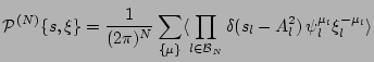
(24) is correct. Now we can easily represent
(24) in terms of the generating functional,
will give zero after the
integration over the unit circle, one can see that LHS=RHS, i.e. that
(24) is correct. Now we can easily represent
(24) in terms of the generating functional,
 |
(23) |
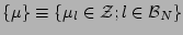
where
 stands for inverse the Laplace
transform with respect to all
stands for inverse the Laplace
transform with respect to all  parameters and
are the angular
harmonics indices.
parameters and
are the angular
harmonics indices.
Note that we could have defined  for all real
  's in which
case obtaining
's in which
case obtaining  would involve finding the Mellin transform of
with respect to all 's. We will see below however that, given
the random-phased initial conditions, will remain zero for all
non-integer 's. More generally, the mean of any quantity which
involves a non-integer power of a phase factor will also be
zero. Expression (26) can be viewed as a result of the
Mellin transform for such a special case. It can also be easily
checked by considering the mean of a quantity which involves integer
powers of
would involve finding the Mellin transform of
with respect to all 's. We will see below however that, given
the random-phased initial conditions, will remain zero for all
non-integer 's. More generally, the mean of any quantity which
involves a non-integer power of a phase factor will also be
zero. Expression (26) can be viewed as a result of the
Mellin transform for such a special case. It can also be easily
checked by considering the mean of a quantity which involves integer
powers of  's.
's.
By definition, in RPA fields all variables  and are
statistically independent and 's are uniformly distributed on
the unit circle. Such fields imply the following form of the
generating functional
and are
statistically independent and 's are uniformly distributed on
the unit circle. Such fields imply the following form of the
generating functional
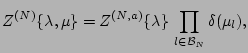 |
(24) |
where
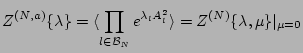 |
(25) |
is an  -mode generating function for the amplitude statistics.
Here, the Kronecker symbol
-mode generating function for the amplitude statistics.
Here, the Kronecker symbol
 ensures independence of the
PDF from the phase factors . As a first step in validating
the RPA property we will have to prove that the generating functional
remains of form (27) up to
ensures independence of the
PDF from the phase factors . As a first step in validating
the RPA property we will have to prove that the generating functional
remains of form (27) up to  and
and
 corrections
over the nonlinear time provided it has this form at
corrections
over the nonlinear time provided it has this form at  .
.
Next: One-mode statistics
Up: Setting the stage II:
Previous: Wavefields with long spatial
Dr Yuri V Lvov
2007-01-23