Probability Distribution Function.

Let us consider a wavefield $a({\bf x}, t)$ in a periodic cube of with side $L$ and let the Fourier transform of this field be $a_l(t)$ where index $l {\in } {\cal Z}^d$ marks the mode with wavenumber $k_l = 2 \pi l /L$ on the grid in the $d$-dimensional Fourier space. For simplicity let us assume that there is a maximum wavenumber $k_{max}$ (fixed e.g. by dissipation) so that no modes with wavenumbers greater than this maximum value can be excited. In this case, the total number of modes is $N = (k_{max} / \pi L)^d$. Correspondingly, index $l$ will only take values in a finite box, $l \in {\cal B}_N \subset {\cal Z}^d$ which is centred at 0 and all sides of which are equal to $k_{max} / \pi L = N^{1/3}$. To consider homogeneous turbulence, the large box limit $N \to \infty$ will have to be taken. ¹

Let us write the complex $a_l$ as $a_l =A_l \psi_l$ where $A_l$ is a real positive amplitude and $\psi_l$ is a phase factor which takes values on ${\cal S}^{1}$, a unit circle centred at zero in the complex plane. Let us define the $N$-mode joint PDF ${\cal P}^{(N)}$ as the probability for the wave intensities $A_l^2$ to be in the range $(s_l, s_l +d s_l)$ and for the phase factors $\psi_l$ to be on the unit-circle segment between $\xi_l$ and $\xi_l + d\xi_l$ for all $l \in {\cal B}_N$. 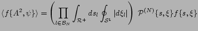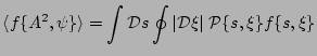In terms of this PDF, taking the averages will involve integration over all the real positive $s_l$'s and along all the complex unit circles of all $\xi_l$'s,

$$\langle f\{A^2, \psi \} \rangle = \left( \prod_{ l {\cal 2 B}_N }... ... S}^{1} } \vert d \xi_l\vert \right) \; {\cal P}^{(N)} \{s, \xi \} f\{s, \xi \}$$ (14)

where notation $f\{A^2,\psi\}$ means that $f$ depends on all $A_l^2$'s and all $\psi_l$'s in the set $\{A_l^2, \psi_l; l {\cal 2 B}_N \}$ (similarly, $\{s, \xi \}$ means $\{s_l, \psi_l; l \in {\cal B}_N \}$, etc). The full PDF that contains the complete statistical information about the wavefield $a({\bf x}, t)$ in the infinite $x$-space can be understood as a large-box limit

$${\cal P} \{ s_k, \xi_k \} = \lim_{N \to \infty} {\cal P}^{(N)} \{s, \xi \},$$

i.e. it is a functional acting on the continuous functions of the wavenumber, $s_k$ and $\xi_k$. In the the large box limit there is a path-integral version of (17),

$$\langle f\{A^2, \psi \} \rangle = \int {\cal D}s \oint \vert{\cal D} \xi\vert \; {\cal P} \{s, \xi \} f\{s, \xi \}$$ (15)

The full PDF defined above involves all $N$ modes (for either finite $N$ or in the $N \to \infty$ limit). By integrating out all the arguments except for chosen few, one can have reduced statistical distributions. For example, by integrating over all the angles and over all but $M$ amplitudes,we have an ``$M$-mode'' amplitude PDF,

$${\cal P}^{(M)}_{j_1, j_2, \dots , j_M} = \left( \prod_{ l \ne j_1... ...\oint_{{\cal S}^{1} } \vert d \xi_m\vert \; \right) {\cal P}^{(N)} \{s, \xi \},$$ (16)

which depends only on the $M$ amplitudes marked by labels $j_1, j_2, \dots , j_M {\cal 2 B}_N$.