Next: Asymptotic Expansions and Closure
Up: Systematic Derivation of the
Previous: Basic Definitions and Evolution
Let us define the cumulant of the  product of spatially dependent
field operators
product of spatially dependent
field operators
 to be the moment of
order from which the appropriate combinations of products of lower
order moments are subtracted so that the resulting expression has the
property that it decays to zero as the separations
to be the moment of
order from which the appropriate combinations of products of lower
order moments are subtracted so that the resulting expression has the
property that it decays to zero as the separations
 become large. The Fourier transforms of these cumulants are
therefore well defined ordinary (as opposed to generalized) functions
and these are the objects
become large. The Fourier transforms of these cumulants are
therefore well defined ordinary (as opposed to generalized) functions
and these are the objects
 with which we deal.
Moreover, if the statistics are exactly Gaussian (namely, Hartree-Fock
like), then all cumulants of order ,
with which we deal.
Moreover, if the statistics are exactly Gaussian (namely, Hartree-Fock
like), then all cumulants of order ,  , are zero. Because these
weakly interacting fermionic systems relax to a near Gaussian state,
the cumulants are the most convenient dependent variables.
, are zero. Because these
weakly interacting fermionic systems relax to a near Gaussian state,
the cumulants are the most convenient dependent variables.
For the two and three particle functions we define the fourth and
sixth order cumulants
 and
and
 respectively by
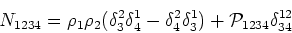 |
(2.10) |
and
The expressions are analogues
to what one would obtain in the classical case. There, the symbols
 and
and  are complex numbers (or c-numbers, as
opposed to operators in the quantum case) and one defines the
cumulants by expanding the fourth order moments into all possible
decompositions; namely
are complex numbers (or c-numbers, as
opposed to operators in the quantum case) and one defines the
cumulants by expanding the fourth order moments into all possible
decompositions; namely
 |
(2.11) |
where angle brackets denote
moments and curly brackets denote the corresponding cumulants. In the
classical case, it is consistent, but not necessary (one can keep the
other terms and discover they play no essential role), to set all
correlations such as
 and
and  equal to zero.
In the quantum case, one also decomposes
equal to zero.
In the quantum case, one also decomposes
 into products of all possible
decompositions. Again, it is consistent, but not necessary, to set
terms such as
into products of all possible
decompositions. Again, it is consistent, but not necessary, to set
terms such as
 and equal
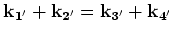
to zero. The resulting decomposition should be consistent with the
anticommutation relations (2.1), from which follows
that
and equal
to zero. The resulting decomposition should be consistent with the
anticommutation relations (2.1), from which follows
that
 . Therefore, certain terms (for example,
 ) are negative in
(2.10-2.11).
) are negative in
(2.10-2.11).
A general algorithm for the decomposition of the  order
expectation value is given in the Appendix.
order
expectation value is given in the Appendix.
Having defined the higher order cumulants, we can now write down the
evolution equations for the cumulant hierarchy. For the purpose of
deriving the QKE, it is sufficient to consider only the equations for
 and
and
 . To obtain the frequency corrections to order
 (
(
 , is a measure of the strength of the coupling
coefficient), we need to consider contributions coming from the
equation for
. In carrying out the analysis on ,
and
, one finds, just as in the classical
case, that certain patterns emerge which allow one to identify the
terms in the equations for the cumulants of arbitrary high order that
gives rise to long time effects. Taking account of these terms gives
the expansions (2.16,2.17) which will be discussed
in the next section. In this section we only write down equations for
and
. They are
, is a measure of the strength of the coupling
coefficient), we need to consider contributions coming from the
equation for
. In carrying out the analysis on ,
and
, one finds, just as in the classical
case, that certain patterns emerge which allow one to identify the
terms in the equations for the cumulants of arbitrary high order that
gives rise to long time effects. Taking account of these terms gives
the expansions (2.16,2.17) which will be discussed
in the next section. In this section we only write down equations for
and
. They are
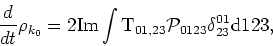 |
(2.12) |
where  denotes the imaginary part and the symbol zero denotes
  , and
, and
on
 , and the
Hartree-Fock self-energy is
, and the
Hartree-Fock self-energy is
At this stage, it is worthwhile pointing out precisely those terms,
underlined in (2.14) that
give rise to the various long term effects:
- The terms that gives rise to particle number transfer in the
QKE are
The reason is
that when one solves for
, one obtains an expression
which contains this term multiplied by
In the long time limit,
Under the operator  in (2.13), the delta-function is
counted twice, and the principal value term cancels. The observant
reader will notice that the QKE can be effectively derived by simply
ignoring all terms in the equation for
in (2.13), the delta-function is
counted twice, and the principal value term cancels. The observant
reader will notice that the QKE can be effectively derived by simply
ignoring all terms in the equation for
 (except
 ) proportional to cumulants of order
greater than two. In the literature, this is called the Hartree-Fock
approximation. What we show in this paper is that, for the magnitude
) proportional to cumulants of order
greater than two. In the literature, this is called the Hartree-Fock
approximation. What we show in this paper is that, for the magnitude
 of the coupling coefficient uniformly (in ) small, the
Hartree-Fock approximation is indeed self consistent when one takes
proper account of the frequency renormalization to order .
of the coupling coefficient uniformly (in ) small, the
Hartree-Fock approximation is indeed self consistent when one takes
proper account of the frequency renormalization to order .
- The order renormalizations to the frequency comes from the
decomposition of sixth order moments such as
 in (2.7). These give rise to
terms in the equation for
which are proportional to
itself. Indeed one obtains one such contribution from
each of the sixth order moments in (2.7) leading to an
expressions in the equation for
equal to
in (2.7). These give rise to
terms in the equation for
which are proportional to
itself. Indeed one obtains one such contribution from
each of the sixth order moments in (2.7) leading to an
expressions in the equation for
equal to
When added to the frequency factor
 , we obtain the term denoted by
 in (2.14). It is not too difficult to see that,
in the equation for every cumulant
in (2.14). It is not too difficult to see that,
in the equation for every cumulant  , there is a term proportional
to
, there is a term proportional
to
and
this gives rise to the first contribution in the renormalization of
the frequency (2.22). In the literature,
is called Hartree-Fock self energy for fourth order
averages.
- The order terms in the renormalization to the
frequency arise from the terms
containing the sixth order cumulants in (2.14). The
equations for the sixth order cumulant contains, in addition to terms
proportional to a product of lower order particle number densities,
terms proportional to
with a factor containing
 .
.
- All other terms are integrals which contain highly oscillatory
factors which, because of the Riemann-Lebesgue lemma, contribute
nothing in the long time limit.
Next: Asymptotic Expansions and Closure
Up: Systematic Derivation of the
Previous: Basic Definitions and Evolution
Dr Yuri V Lvov
2007-01-31