Asymptotic Expansions and Closure

We take advantage of the small parameter, the strength $\epsilon$ of the coupling coefficient and make the formal substitution $T_{12,34}\to\epsilon T_{12,34}$. We expand all cumulants $Q_{N}$ in an asymptotic expansion

$$Q_2\equiv \rho _k=n_k+\epsilon Q_{2}^{(1)}+\epsilon ^2 Q_{2}^{(2)}+...$$ (2.13)

and

$$Q_{N}(k_1,k_2,k_3...k_N;t)= Q_N^{(0)}+\epsilon Q_N^{(1)}+\epsilon ^2 Q_N^{(2)}+ ... N>2$$ (2.14)

Because of resonant interactions, these asymptotic expansions will be nonuniform in time. Namely, terms proportional to $\epsilon t$, $\epsilon ^2 t$, etc., will appear in $Q_{N}$. These terms are removed and the asymptotic expansions (2.16,2.17) rendered well ordered by allowing corrections to the time dependence of the leading order cumulants $n_k$, $Q^{(0)}_N, N>2$. We make the ansatz

$$\frac{\partial n_k}{\partial t} = \epsilon ^2 F_2^{(2)}+...$$ (2.15)

$$\frac{\partial Q^{(0)}_{1,2,..N}}{\partial t} = i(\omega _1+\omega _2+... - \omega _{N})Q^{(0)}_{1,2,..N}+ \epsilon F_{1,2,..N}^{(1)}+\epsilon ^2 F_{1,2,..N}^{(2)}+...$$

and choose $F_2^{(2)}, \ F_N^{(1)}, F_N^{(2)} ... N>2$ in order to keep (2.16,2.17) asymptotically uniform for times $\omega _{k_0}t=O(\epsilon ^{-2})$. Equations (2.18) and (2.19) describe the long time behavior of the system.

This method goes by many names, averaging, multiple time scales etc., familiar to nonlinear physicists (see, e.g., [3],[19]-[21]). It will turn out that $F_2^{(2)}$ depends only on $n_k$ itself leading to a closed equation for the particle number, the QKE. It will also turn out that $F_N^{(1)}, F_N^{(2)}, N>2$ are simply products of ${Q^{(0)}_N}$ with a function of $n_k$, which is the symmetric sum of $N$ components. This means that the resulting equations (2.19) are easily solved by simply renormalizing the frequency.

The quantum kinetic equation is given by

$$\frac{\partial} {\partial t}n_{k}\equiv\epsilon ^2F_2^{(2)}= (4\e... ...'})) \cr \times( n_{2'}n_{3'}(1-n_{1'}-n_{k})+ n_{k}n_{1'}(n_{2'}+n_{3'}-1))) .$$ (2.16)

where the Hartree Fock self-energy is

$$\tilde \Delta ^{1'2'}_{3'4'}=\omega _{1'}+\omega _{2'}-\omega... ...t((T_{1'1,11'}+ T_{2'1,12'}-T_{3'1,13'}-T_{4'1,14'})n_1\right).$$

From the form of (2.20), it is clear that number density is redistributed by binary particle collisions which satisfy momentum and energy conservation. In particular, exchange of particle number (momenta, energy) is associated with particles whose momenta and energies lie on the resonant manifold defined to a good approximation by

$${\bf k_1}+{\bf k_2}-{\bf k_3}-{\bf k_4}=0, \ \omega _{k_1}+\omega _{k_2}-\omega _{ k_3}-\omega _{k_4}=0.$$ (2.17)

The evolution equation for $Q_{1'2'...N}^{(0)}$ can be written

$$\frac{\partial \ln{Q_{12..N}^{(0)}}}{\partial t} = i \left(\sum_{i=1}^{N/2}\Omega _{i}-\sum_{i=N/2+1}^{N}\Omega ^*_{i} \right),$$

$$\Omega _{k'} = \omega _{k'}+2\epsilon \int d1 n_1 T_{1'1,11'}$$

$$+2 \epsilon ^2 \int d123 \left( n_1+n_2 n_3-n_1 n_3- n_1 n_2 \right) T^2_{k'123}\delta ^{k'1}_{23}$$

$$\times \left(P(\frac{1}{\tilde\Delta^{k'1}_{23}})+ i \pi {\rm {sgn}}(t)\delta ( \tilde\Delta^{k'1}_{23})\right)$$

which can be interpreted as a complex frequency renormalization.

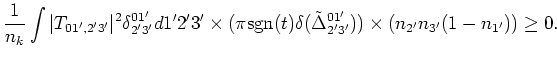
We can calculate the sign of $\rm Im\Omega$ once $n_k$ reaches its steady (equilibrium) state. For steady state $\dot n_k=0$ we rewrite the QKE (2.20) as

$$\int \vert T_{01',2'3'}\vert^2\delta ^{01'}_{2'3'}d1'2'3'\times (... ...elta^{01'}_{2'3'})) \cr \times( n_{2'}n_{3'}-n_{1'}n_{2'}-n_{1'}n_{3'}+n_{1'} )$$

$$=$$

$$\frac{1}{n_k}\int \vert T_{01',2'3'}\vert^2\delta ^{01'}_{2'3'}d1... ...t)\delta (\tilde\Delta^{01'}_{2'3'})) \cr \times( n_{2'}n_{3'}(1-n_{1'}))\ge 0.$$ (2.18)

The LHS of the above equation is the imaginary part of $\Omega _k$. Observe that, because $\rm Im\Omega _k\ge 0$, the leading order approximation to the $N^{th}$ ($N\ge 2$) order cumulant decays with time. This means that the memory of (smooth) initial states is gradually forgotten.

We want to make two very important points which are often overlooked. While the leading order contributions (which at $t=0$ is the initial state multiplied by an oscillatory factor) to the $N^{th}$ order cumulants for $N>2$ play no role in the long time behavior of the system and indeed slowly decay, higher order (in $\epsilon$) contributions do not disappear in the long time limit. The system retains a weakly non Gaussian character which is responsible for and essential for particle number and energy transfer. For example, in the long time limit, the order $\epsilon$ fourth order cumulant has the quasi stationary contribution (the terms with higher order cumulants asymptote to zero by means of phase mixing and the Riemann-Lebesgue lemma)

$$\nonumber {{\cal{P}}}_{1'2'3'4'}^{(1)}(t)= 2i T_{4'3',2'1'}(n... ...3'}+n_{4'}-1)) \times A_t(\tilde\Delta^{1'2'}_{3'4'}) \nonumber$$

where

$$A_t(x)=\int\limits_0^t d \tau \exp[i x \tau ].$$

Because $\lim_{t\to\infty} A_t(x)=\pi {\rm {sgn}}t \cdot \delta (x)+i P(\frac{1}{x}),$ in the limit $t\to\infty$,

$${{\cal{P}}}_{1'2'3'4'}^{(1)}(t)\to 2i T_{4'3',2'1'}(n_{3'}n_{4'}(... ...ta^{1'2'}_{3'4'})+i P(\frac{1} {\tilde\Delta^{1'2'}_{3'4'}}) \right) .\nonumber$$

Thus, in the long time limit, the order $\epsilon$ contribution ${{\cal{P}}}_{1234}^{(1)}$ to the fourth order cumulant is not smooth but is given by a sum of generalized functions represented by the Dirac delta function and the Cauchy Principal value. We may therefore legitimately ask: in what sense is the asymptotic series (2.16,2.17) well ordered if it contains terms which are products of powers of $\epsilon$ with generalized functions? The answer is that to analyze properly the asymptotic behavior of the system, we must always revert to physical space and look at the corresponding asymptotic expansion for the cumulants $\{\psi^\dagger({\bf r})\psi^\dagger({\bf r'})\psi({\bf r''})\psi({\bf r'''})\}$ connected with fourth order expectation values of the field operators. These objects, which decay to zero as the separations ${\bf r'}-{\bf r}, {\bf r''}-{\bf r}, \ {\bf r'''}-{\bf r}$ tend to infinity, are simply the Fourier transform of ${{\cal{P}}}_{kk'k''k'''}$. We can also show that no terms worse than single delta functions occur (or products of delta functions which have their support on different resonant submanifolds) at later powers of $\epsilon$ so that the resulting asymptotic expansion for the spatial cumulants is indeed well ordered.

The second important point concerns the reversibility or rather the retracebility of solutions of (2.20,2.22). In the derivation of (2.20,2.22), we assumed that the initial cumulants were sufficiently smooth so that integrals over momentum space of multiplications of the initial values of $Q_N$ by $\exp(-i(\omega _1+.... - \omega _N)t)$ tend to zero in the asymptotic limit. However, it is clear from (2.22) that the regenerated cumulants have terms of higher order in $\epsilon$ which are not smooth and indeed have their (singular) support precisely on the resonant manifold which is the exponent of the oscillatory exponential. What would happen, then, if one were to redo the initial value problem from a later time $t_1=O(\epsilon ^{-2})$, either positive or negative, after which the fourth order cumulant had developed a nonsmooth part? On the surface, it would seem that the ${\rm {sgn}}$ term in (2.22) would be ${\rm {sgn}}(t-t_1)$ so that, at every time $t_1$, there would be a discontinuity in the slope of $n_k(t)$. But that is not the case. If one accounts for the nonsmooth behavior (2.22) in the new initial value for ${{\cal{P}}}_{1234}^{(1)}$, then one gets additional terms in (2.22) which give exactly the same collision integral but with the factor $({\rm {sgn}}t-{\rm {sgn}}(t-t_1))$. Adding the two contributions, we find the QKE is exactly the same as the one derived beginning at $t=0$. It is not that the point $t=0$ is so special. Rather, there is a range of times $t$, $-\epsilon ^{-2}\ll\omega _{k_0}t\ll\epsilon ^{-2}$ such that, if one begins anywhere within this range, an initially smooth distribution stays smooth. But once the limit $t\to\infty$, $\epsilon ^2 t$ finite, is taken, an irreversibility and nonsmoothness in the cumulants is introduced.

In a very real sense, then, the infinite dimensional Hamiltonian system acts as if there is an attracting manifold (an inertial or generalized center manifold in the modern vernacular) in its phase space to which the system relaxes as $\omega _{k_0}t\to O(\epsilon ^{-2})$ (in either time direction) on which the slow dynamics is given by the closure equations (2.20),(2.22). On this attracting manifold, the higher order cumulants are essentially slaved to the particle number density and their frequencies are renormalized by contributions which also depends on particle number density. The attenuation in this case is due to losses to the heat bath consisting of all momenta which do not lie on a resonance manifold associated with ${\bf k}$.