Next: Cumulants and their evolution.
Up: Systematic Derivation of the
Previous: Systematic Derivation of the
We start from the Hamiltonian (1.1) of a spatially homogeneous
system of particles with binary interactions. Here,
 is the energy level of momentum state
  (for example, in
semiconductors, the parabolic band approximation is given by
(for example, in
semiconductors, the parabolic band approximation is given by
 ) where is a d-dimensional wave vector, and
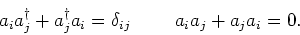
 are fermionic creation/annihilation operators
fulfilling the anticommutation relations,
are fermionic creation/annihilation operators
fulfilling the anticommutation relations,
 |
(2.1) |
We include the size of the system in the
definition of the interaction matrix element  . We
introduce for convenience the short hand notation:
. We
introduce for convenience the short hand notation:
 ,
,
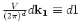 , and
, and
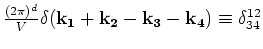 ,
,  . The
Hamiltonian now reads
. The
Hamiltonian now reads
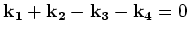
If one interchanges the indices  and
and  or
or  and
and  in the above expression and uses the fact that the Hamiltonian
is Hermitian, the following properties hold:
in the above expression and uses the fact that the Hamiltonian
is Hermitian, the following properties hold:
In the Heisenberg picture, the
equations of motion are
![\begin{displaymath}\dot a_k = i[H,a]_-
\end{displaymath}](img60.png) |
(2.2) |
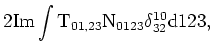
which give
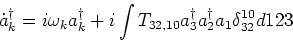 |
(2.3) |
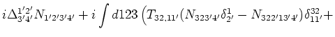
and
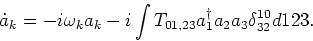 |
(2.4) |
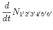
From the Heisenberg equations of motion, one can now
derive the BBGKY hierarchy of equations for the normal ordered
expectations values. The first three
are,
where
Here, the expectation value is taken with respect to an arbitrary
initial state  , i.e.,
In the definitions of these
 order
expectation values, the first
order
expectation values, the first  indices correspond to creation
operators and the last
indices correspond to annihilation operators. The number of
creation and number of annihilation operators are equal to each other
because the Hamiltonian (1.1) conserves number of particles. The
fact that the right hand sides of (2.9) are zero on
indices correspond to creation
operators and the last
indices correspond to annihilation operators. The number of
creation and number of annihilation operators are equal to each other
because the Hamiltonian (1.1) conserves number of particles. The
fact that the right hand sides of (2.9) are zero on
 ,
,
 respectively is a direct consequence of the spatial
homogeneity of the system. This means that the
respectively is a direct consequence of the spatial
homogeneity of the system. This means that the  order moment of
the spatially dependent field operators
order moment of
the spatially dependent field operators
 , the generalized Fourier transforms of the
creation and annihilation operators
, the generalized Fourier transforms of the
creation and annihilation operators
 , depends only on the relative
spacing; i.e. on the differences of the coordinates
, depends only on the relative
spacing; i.e. on the differences of the coordinates
 .
.
Next: Cumulants and their evolution.
Up: Systematic Derivation of the
Previous: Systematic Derivation of the
Dr Yuri V Lvov
2007-01-31