


Next: Results
Up: Energy spectra of internal
Previous: Hamiltonian formalism for internal
Numerical methods
Table 1:
Numerical parameters.
| |
modes |
 ( (
 rad/sec) rad/sec) |
 ( ( kg/m kg/m ) ) |
forcing |
initial condition |
| I |
 |
 |
2.7 |
none |
GM |
| II |
 |
|
2.7 |
 |
white noise |
| III |
 |
 |
5 |
 |
white noise |
| IV |
|
 |
5 |
|
white noise |
| V |
|
|
2.7 |
none |
GM w/o long waves |
In direct numerical simulations,
we add external forcing and hyper-viscosity
to the canonical equation (5),
as forcing and damping are needed to achieve statistically steady states.
Thus the resulting dynamic equation is given by
In the simulations,
the linear terms,
which are a linear dispersion term and a dissipation term,
 ,
are explicitly calculated.
The nonlinear terms,
,
are explicitly calculated.
The nonlinear terms,
 , derived from the nonlinear parts of the canonical equation (5) with Hamiltonian (6)
are obtained by a pseudo-spectral method with the phase shift
under the periodic boundary conditions for all three directions.
The external forcing,
, derived from the nonlinear parts of the canonical equation (5) with Hamiltonian (6)
are obtained by a pseudo-spectral method with the phase shift
under the periodic boundary conditions for all three directions.
The external forcing,  , is implemented
by fixing the amplitudes of several small wavenumbers to be constant in time.
The dissipation is also added as
, is implemented
by fixing the amplitudes of several small wavenumbers to be constant in time.
The dissipation is also added as
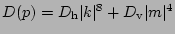 .
Here,
.
Here,
 and
and
 are chosen
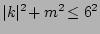
so that the dissipation is effective for wavenumbers
larger than the half of maximum wavenumbers.
The wavenumbers are discretized as
are chosen
so that the dissipation is effective for wavenumbers
larger than the half of maximum wavenumbers.
The wavenumbers are discretized as
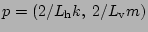 , where
 and
are
horizontal periodic length and vertical period in the isopycnal coordinates,
and
and
are
horizontal periodic length and vertical period in the isopycnal coordinates,
and  and
and  are integer-valued wavenumbers afterward.
Time-stepping is implemented with the fourth-order Runge-Kutta method.
In all the simulations,
the buoyancy frequency and horizontal period are fixed at
are integer-valued wavenumbers afterward.
Time-stepping is implemented with the fourth-order Runge-Kutta method.
In all the simulations,
the buoyancy frequency and horizontal period are fixed at  rad/sec and
 m, respectively.
We perform a series of five numerical experiments that are listed in Table 1.
The total energy per unit periodic box of all the numerical experiments except Run II
is around  J/(kg
J/(kg  m
m ) which is characteristic of real oceans.
The total energy in the Run II is around
) which is characteristic of real oceans.
The total energy in the Run II is around
 J/(kg m).
Two-dimensional energy spectra are measured in the shell of radius  as
as
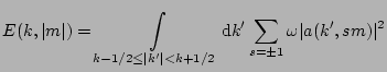 |
|
|
(20) |
 |
|
|
(21) |
Integrated energy spectra are defined as
 and
and
 .
Cross-sectional spectra,
.
Cross-sectional spectra,  and
and  ,
are obtained from the two-dimensional energy spectra
as a function of isopycnal wavenumbers
along a certain density wavenumber
and
as a function of density wavenumbers
along a certain isopycnal wavenumber , respectively.
,
are obtained from the two-dimensional energy spectra
as a function of isopycnal wavenumbers
along a certain density wavenumber
and
as a function of density wavenumbers
along a certain isopycnal wavenumber , respectively.
In general in real oceans
only integrated spectra,
 obtained from time series and
 from vertical series,
can be measured.
Then the two-dimensional spectrum,
from vertical series,
can be measured.
Then the two-dimensional spectrum,  , is composed from integrated spectra.
To do it,
the assumption of separability of two-dimensional spectra is made.
Namely, the functional form,
, is composed from integrated spectra.
To do it,
the assumption of separability of two-dimensional spectra is made.
Namely, the functional form,
 ,
is assumed.
As we will see below in our numerical simulations,
our resulting spectra are not always separable.
Such non-separability is also observed in the real oceans (Polzin, 2007).
Note that the power-law exponents of one-dimensional spectra and those of two-dimensional spectra do not always coincide in our direct numerical simulation,
as explained below.
We do not have any means to see whether this observation will also hold in the real ocean.
,
is assumed.
As we will see below in our numerical simulations,
our resulting spectra are not always separable.
Such non-separability is also observed in the real oceans (Polzin, 2007).
Note that the power-law exponents of one-dimensional spectra and those of two-dimensional spectra do not always coincide in our direct numerical simulation,
as explained below.
We do not have any means to see whether this observation will also hold in the real ocean.
Figure 1:
Run I. Cross-sectional spectra
of GM spectrum as the initial condition (left)
and
of energy spectrum after about 35 hours (right).
Significant differences in the region  indicates that GM spectrum is not statistically steady.
|
|
Next: Results
Up: Energy spectra of internal
Previous: Hamiltonian formalism for internal
Dr Yuri V Lvov
2007-06-26

![\includegraphics[scale=0.71]{gm0_psfrag.eps}](img104.png)
![\includegraphics[scale=0.71]{gm4_psfrag.eps}](img105.png)