Results

In the first numerical experiment, Run I of Table 1, we examine statistical stability of the GM spectrum of a freely decaying system, i.e. without external forcing. The GM spectrum with the cut-off in large isopycnal and density wavenumbers is employed as the initial energy spectrum. The cut-off is introduced to avoid decreasing accuracy of the pseudo-spectral method. The initial phases of complex amplitude, $a(\bldp)$, are given by uniformly distributed random numbers in $[ 0,2\upi )$. Figure 1 shows the initial spectrum and the energy spectrum after about 35 hours in ocean time. If the GM spectrum were to be a universal steady state for this numerical run, it would change very little. Instead, the density exponents rapidly change from $-1$ to $-2$ only after $1.5$ days. This spectral change occurs faster than dissipation affects with timescale estimated to be about 50 days at $\vert m\vert=32$. Therefore it appears that the GM spectrum is not a stable universal spectrum in the wavenumber region $16 < \vert m\vert < 64$ at least for this numerical experiment. This suggests that the diffusion approximation of the kinetic equation (McComas, 1977; McComas & Müller, 1981), which predicts that energy spectra are rapidly relaxed to the GM spectrum, may not be fully appropriate.

Figure 2: Run II. Two-dimensional energy spectrum $E(k,\vert m\vert)$. The contours are plotted every powers of ten from $10^{-10}$ to $1$. The straight line from the origin shows the wavenumbers $\omega =2f$. The inset is the enlargement near the origin.

Hoping to find a statistically steady state, we then performed a forced-damped simulation, Run II (see Table 1). The external forcing is added to 24 small wavenumbers whose frequencies are close to $3f$ such that $(\bldk, m) = (\pm 1, 0, \pm 2)$, $(0, \pm 1, \pm 2)$, $(\pm 1, \pm 1, \pm 3)$, $(\pm 2, 0, \pm 4)$ and $(0, \pm 2, \pm 4)$. The two-dimensional energy spectrum in near statistically steady state obtained in this simulation is shown in Fig. 2. We observe that there is a significant energy accumulation around $k \sim 1$, i.e. the horizontally longest waves. Note that linear frequency given by dispersion relation is exactly $f$ when $k=0$. Similarly, accumulation of energy around $k \sim 1$ corresponds to accumulation of energy in near-inertial frequencies. This is precisely what happens in the ocean! Indeed all versions of the GM spectra have an integrable singularity in near-inertial frequencies such as $1/\sqrt{\omega^2 - f^2}$ (Garrett & Munk, 1972,1975,1979), indicating significant energy contents in near-inertial waves. Such an accumulation can be explained quantitatively as a result of a parametric subharmonic instability (Furuich, Hibiya & Niwa, 2005) which arises in small isopycnal wavenumbers.

Figure: Run II. Integrated energy spectra $\overline{E}_{\mathrm{int}}(k)$ and $\overline{E}_{\mathrm{int}}(\vert m\vert)$, and cross-sectional energy spectra $E_m(k)$ and $E_k(\vert m\vert)$. GM spectrum has $k^{-2} \vert m\vert^{-1}$ in large isopycnal and density wavenumbers. The cross-sectional spectra are shown every four curves for visibility.

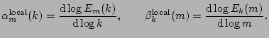
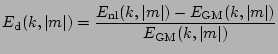
Figure 3 shows integrated spectra, $\overline{E}_{\mathrm{int}}(k)$ and $\overline{E}_{\mathrm{int}}(\vert m\vert)$, and cross-sectional spectra, $E_m(k)$ and $E_k(\vert m\vert)$ obtained from two-dimensional energy spectrum shown in Fig. 2. The integrated spectra are $\overline{E}_{\mathrm{int}}(k) \propto k^{-1.98 \pm 0.02}$ and $\overline{E}_{\mathrm{int}}(\vert m\vert) \propto \vert m\vert^{-1.33 \pm 0.31}$. The exponents are not too far from the large-wavenumber self-similar form of GM spectrum, that is $k^{-2} \vert m\vert^{-1}$. The exponents are obtained with the least-square method in the intervals of $k \in [8,128]$ for $\overline{E}_{\mathrm{int}}(k)$ and that of $\vert m\vert \in [4,32]$ for $\overline{E}_{\mathrm{int}}(\vert m\vert)$.

Figure 4: Run II. Power-law exponents of each cross-sectional spectrum. left: $\alpha (\vert m\vert)$, which are the exponents of cross-sectional energy spectra $E_{m}(k)$, right: $\beta (k)$, which are the exponents of cross-sectional energy spectra $E_{k}(\vert m\vert)$. The exponents of integrated spectra, $\alpha_{\mathrm{int}}=-1.98$ and $\beta_{\mathrm{int}}=-1.33$, are also shown.

Figure 5: Run II. Local power-law exponents. The exponents are derived from $E_{m=16}(k)$, $E_{m=48}(k)$, $E_{k=32}(m)$ and $E_{k=96}(m)$.

Figure 4 shows power-law exponents of each cross-sectional spectrum, $\alpha (\vert m\vert)$ and $\beta (k)$, which are obtained by fitting $E_{m}(k) \propto k^{\alpha(\vert m\vert)}$ in $k \in [16,128]$ and $E_{k}(m) \propto \vert m\vert^{\beta(k)}$ in $\vert m\vert \in [16,64]$. The exponents of integrated spectra, $\alpha_{\mathrm{int}}=-1.98$ and $\beta_{\mathrm{int}}=-1.33$, are also shown in Fig. 4. Note that the fitted regions of cross-sectional spectra are different from those of integrated spectra. The integrated spectra have different exponents from the ones of cross-sectional spectra in inertial region since the integrated spectra are greatly affected by the accumulation in small isopycnal or density wavenumbers. Especially, the discrepancy is clear in the density exponent $\beta$ because of the strong accumulation around $k \sim 1$. Apparently, the cross-sectional exponents are not constant. Therefore, the energy spectrum of this numerical simulation cannot be accurately fitted by double-power functions. It also appears that this spectrum is non-separable. Moreover, in contrast to the integrated spectra, both cross-sectional spectra have much steeper exponents, $\alpha, \beta \sim -3.5$, than the GM spectrum has in large isopycnal and density wavenumbers considered as inertial region. Local exponents of cross-sectional spectra are defined as

$$\alpha_m^{\mathrm{local}}(k) = \frac{\mathrm{d} \log E_m(k)}{\mat... ...\beta_k^{\mathrm{local}}(m) = \frac{\mathrm{d} \log E_k(m)}{\mathrm{d} \log m}.$$ (22)

We observe that the local exponents are also close to $-3.5$ in large isopycnal and density wavenumbers shown in Fig. 5, although the local exponents, $\alpha_m^{\mathrm{local}}(k)$ in particular, are jagged. Poor redistribution of energy from the accumulation of energy in small isopycnal wavenumbers and that in small density wavenumbers can make steeper spectra as well.

Figure 6: Run III. Integrated and cross-sectional spectra when the accumulation of energy around the horizontally longest waves is weak.

Figure 7: Run IV. Integrated and cross-sectional spectra when the accumulation of energy around the horizontally longest waves is moderate.

Figure 8: Run III. Power-law exponents when the accumulation of energy around the horizontally longest waves is weak.

Figure 9: Run IV. Power-law exponents when the accumulation of energy around the horizontally longest waves is moderate.

Next, we investigate the influence of this accumulation of energy on inertial wavenumbers. To achieve this goal, we perform two numerical runs III and IV in Table 1. These two runs are different by value of inertial frequencies $f$ (see Table 1). The difference of values of inertial frequencies influences the rate of formation of the accumulation around the horizontally longest waves. After about $10^3$ days from the initial time when all the wavenumbers have extremely small energy, the system is still transient and the accumulation of energy around the horizontally longest waves has not developed strongly. The timescales of the formation of the accumulation, which are determined by nonlinear interactions among the long waves, are much longer than those of the inertial wavenumbers. The energy spectrum of the case with $f=0.25 \times 10^{-4}$rad/sec has only weak accumulation since all the forced wavenumbers have frequencies greater than $4f$, far from the linear frequencies of the wavenumbers that constitute the accumulation. The energy spectrum of the case with $f=10^{-4}$rad/sec has moderate accumulation, which is stronger than that of the case with $f=0.25 \times 10^{-4}$rad/sec and is weaker than that of Run II.

The integrated and cross-sectional spectra and their power-law exponents after $10^3$ days are shown in Figs. 6, 7, 8 and 9. The least-square fitting to obtain the power-law exponents is made in the intervals of $k,m \in [8,40]$. When the accumulation of energy around the horizontally longest waves is weak enough, the energy spectrum is close to the double-power $E(k,m) \propto k^{-2} \vert m\vert^{-2.5}$ in large isopycnal and density wavenumbers. On the other hand, the energy spectrum does not have double-power laws in the region when the accumulation is moderate. It is caused by contamination of the inertial region due to the accumulation. Another double-power law $E(k,m) \propto k^{-2} \vert m\vert^{-2}$ appears in small isopycnal and density wavenumbers. Again, we point out that the exponents of cross-sectional spectra are also sufficiently different from those of the integrated spectra and the GM spectrum. Therefore, in combination with Run II, it appears that the accumulation of energy around the horizontally longest waves strongly affects statistical properties in the inertial region.

Figure 10: Relative difference between energy spectra after about $1.5$ days developed from GM spectrum with and without energy in small isopycnal wavenumbers $E_{\mathrm{d}}(k,\vert m\vert)$.

To further illustrate this point, and to investigate the importance of nonlocal interactions in the wavenumber space, we perform Run V of Table 1. There we choose the initial condition same as the Run I but with no energy in $k<3$ and $\vert m\vert < 16$. The energy spectrum after about $1.5$ days is denoted by $E_{\mathrm{nl}}(k,\vert m\vert)$. The energy spectrum developed from the GM spectrum in Run I that is shown in Fig. 1(right) is denoted by $E_{\mathrm{GM}}(k,\vert m\vert)$. Figure 10 shows the relative difference defined as

$$E_{\mathrm{d}}(k,\vert m\vert) = \frac{E_{\mathrm{nl}}(k,\vert m\vert) - E_{\mathrm{GM}}(k,\vert m\vert)}{E_{\mathrm{GM}}(k,\vert m\vert)}$$ (23)

$$end{tex2html_deferred}, .$$ (24)

The wavenumbers different in initial conditions appear as a black rectangle in bottom left in Fig. 10. If the nonlocal interactions with the accumulation of energy around the horizontally longest waves were not dominant, the relative difference in Fig. 10 would be small or slightly negative in inertial wavenumbers since the nonlinear interactions try to compensate the defect in the small wavenumbers. Instead, $E_{\mathrm{nl}}(k,\vert m\vert)$ has about 50% more energy in $10 \lesssim \vert m\vert \lesssim 40$ drawn in white and less energy transfer to the dissipation region in $\vert m\vert \gtrsim 80$. This suggests that small wavenumbers in the accumulation of energy make energy transfer from small density wavenumbers to large density wavenumbers in the inertial region. Energy transfer to large density wavenumbers is qualitatively consistent to the induced diffusion (McComas, 1977; McComas & Müller, 1981).