Next: Numerical methods
Up: Energy spectra of internal
Previous: Introduction
Equations of motion for incompressible stratified fluid
(i.e. conservation of horizontal momentum, hydrostatic balance, mass
conservation and the incompressibility constraint)
under the assumption of zero potential vorticity
in the isopycnal coordinates,  ,
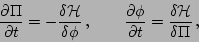
can be written as a pair of canonical
Hamiltonian equations,
,
can be written as a pair of canonical
Hamiltonian equations,
 |
(1) |
where
 is the fluctuation of stratification profile
around the mean,
is the fluctuation of stratification profile
around the mean,  ,
and
,
and  is the isopycnal velocity potential.
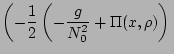
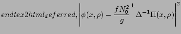
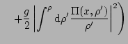
The Hamiltonian is the sum of kinetic and potential energies,
is the isopycnal velocity potential.
The Hamiltonian is the sum of kinetic and potential energies,
(see Lvov & Tabak (2004) for complete details).
The differential operators on the isopycnal surfaces,
 and
and
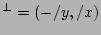 ,
are the horizontal gradient operator and the rotation operator, respectively.
Also,
,
are the horizontal gradient operator and the rotation operator, respectively.
Also,  is the acceleration of gravity,
 is the buoyancy (Brunt-Väisälä) frequency,
 is the inertial frequency due to the rotation of the Earth,
and
is the inertial frequency due to the rotation of the Earth,
and  is the mean density.
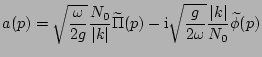
We then perform Fourier transformation and canonical transformation to
the field variable,  , as
, as
 |
|
|
(6) |
 |
|
|
(7) |
with linear coupling of the Fourier components of the stratification profile,
 ,
and the horizontal velocity potential,
,
and the horizontal velocity potential,
 .
The three-dimensional wavenumber,
.
The three-dimensional wavenumber,  , consists of
a two-dimensional horizontal wavenumber in the isopycnal surface,
, consists of
a two-dimensional horizontal wavenumber in the isopycnal surface,  ,
and a vertical density wavenumber,
,
and a vertical density wavenumber,  .
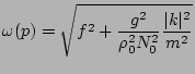
The linear frequency is given by the dispersion relation,
.
The linear frequency is given by the dispersion relation,
 |
|
|
(8) |
 |
|
|
(9) |
The usual vertical wavenumber,  , and the density wavenumber, , are
related as
, and the density wavenumber, , are
related as
 .
The buoyancy frequency, ,
and the inertial frequency, , are assumed to be constants.
.
The buoyancy frequency, ,
and the inertial frequency, , are assumed to be constants.
Then, the equations of motion (1) are rewritten as a
canonical equation,
 |
|
|
(10) |
with the standard Hamiltonian of three-wave interactive system,
 |
 |
 |
(11) |
 |
|
|
|
 |
|
|
(12) |
 |
|
 |
(13) |
 |
|
|
|
|
|
|
(14) |
|
|
 |
(15) |
|
|
|
(16) |
Here,
 is the functional derivative
with respect to
is the functional derivative
with respect to
 that is the complex conjugate of
and the abbreviation c.c. denotes complex conjugates.
Matrix elements,
that is the complex conjugate of
and the abbreviation c.c. denotes complex conjugates.
Matrix elements,
 and
and
 , have exchange symmetries such that
 and
and
 .
.
Next: Numerical methods
Up: Energy spectra of internal
Previous: Introduction
Dr Yuri V Lvov
2007-06-26