Next: Bibliography
Up: Interactions of renormalized waves
Previous: Conclusions
Limiting behaviors of  for the thermalized
  -FPU chain
We change variables
 in the
Hamiltonian (29) for -FPU to obtain
in the
Hamiltonian (29) for -FPU to obtain
![$\displaystyle H(p,y)=\sum_{j=1}^N\left[\frac{1}{2}p_j^2+\frac{1}{2}y_j^2+\frac{\beta}{4}y_j^4\right].$](img365.png) |
|
|
(74) |
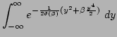
Next, we compute the pdf's for the momentum and displacement.
Any  is distributed with the Gaussian pdf
 and any
  is distributed with the
pdf
is distributed with the
pdf
 , where
  and
and
 are the normalizing constants. As we have discussed, the
renormalization factor of the -FPU system in thermal
equilibrium is given by Eq. (25), and its approximation via
the self-consistency argument
are the normalizing constants. As we have discussed, the
renormalization factor of the -FPU system in thermal
equilibrium is given by Eq. (25), and its approximation via
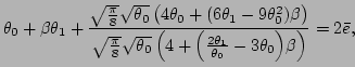
the self-consistency argument  is given by
Eq. (52). Here, we compare the behavior of both formulas
in two limiting cases, i.e., the case of small nonlinearity
is given by
Eq. (52). Here, we compare the behavior of both formulas
in two limiting cases, i.e., the case of small nonlinearity
 and the case of strong nonlinearity
 . We will use the following expressions for
the average density of kinetic, quadratic potential and quartic
potential parts of the total energy of the system
. We will use the following expressions for
the average density of kinetic, quadratic potential and quartic
potential parts of the total energy of the system
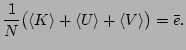
In a
canonical ensemble, the temperature of a system is given by the
temperature of the heat bath. By identifying the average energy
density of the system with
 in our simulation (a
microcanonical ensemble), we can determine
in our simulation (a
microcanonical ensemble), we can determine  as a function of
 and by the following equation
 |
|
|
(78) |
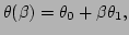
We start with
the case of small nonlinearity
. Suppose in the
first order of the small parameter the temperature has the
following form
 |
|
|
(79) |
where
 and
and
 . We find the values of
  and
and
 using the constraint (A5). We use the following
expansions in the small parameter
using the constraint (A5). We use the following
expansions in the small parameter
| |
|
 |
|
| |
|
 |
(80) |
| |
|
 |
|
| |
|
 |
(81) |
| |
|
 |
|
| |
|
 |
(82) |
Then, in the first order in , Eq. (A5)
becomes
and we obtain
 and
and
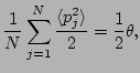
 . Therefore, for
the average kinetic energy density, we have
. Therefore, for
the average kinetic energy density, we have
 |
|
|
(83) |
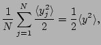
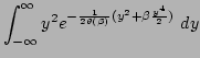
and, for the average quadratic potential energy density, we
have
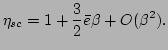
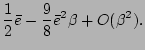
Finally, we obtain Eq. (53), i.e., for small
 |
|
|
(85) |
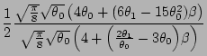
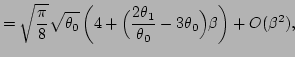
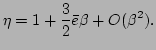
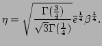
Similarly, from Eq. (52), we find the small limit
of the approximation
Now, we
consider the case of strong nonlinearity
.
From Eq. (A5), we conclude that temperature in the large
limit, which we denote as
 , stays bounded, i.e.,
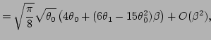
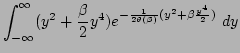
 and, in the limit of large , we obtain for
Eq. (A5)
and, in the limit of large , we obtain for
Eq. (A5)
 |
|
|
(86) |
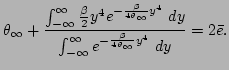
After performing the integration, we obtain
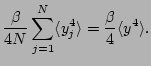
 and the average kinetic energy density becomes
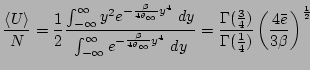
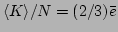 . For the average quadratic potential energy
density, we have
. For the average quadratic potential energy
density, we have
 |
|
|
(87) |
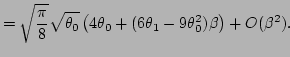
For the renormalization factor, we obtain the following large
scaling
 |
|
|
(88) |
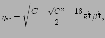
Similarly, for the approximation of , we obtain
 ,
,
 , and
, and
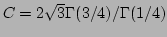 . Therefore, the large
scaling of becomes
. Therefore, the large
scaling of becomes
 |
|
|
(89) |
which yields Eq. (54).
Next: Bibliography
Up: Interactions of renormalized waves
Previous: Conclusions
Dr Yuri V Lvov
2007-04-11