


Next: Dispersion relation and resonances
Up: Interactions of renormalized waves
Previous: Renormalized waves
Numerical study of the  -FPU chain
Since its introduction in the early 1950s, the
study of the FPU lattice [13] has led to many great
discoveries in mathematics and physics, such as soliton
theory [3]. Being non-integrable, the FPU system also became
intertwined with the celebrated Kolmogorov-Arnold-Moser
theorem [11]. Here, we extend our results of the thermalized
-FPU chain, which were briefly reported in [12].
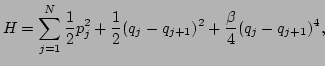
The Hamiltonian of the -FPU chain is of the form
 |
|
|
(29) |
where is a parameter that characterizes the strength of
nonlinearity.
The canonical equations of motion of the -FPU chain are
To
investigate the dynamical manifestation of the renormalized
dispersion
 of
of
 , we numerically integrate
Eq. (30). Since we study the thermal equilibrium
state [14,15,16,17] of the -FPU
chain, we use random initial conditions, i.e.,
, we numerically integrate
Eq. (30). Since we study the thermal equilibrium
state [14,15,16,17] of the -FPU
chain, we use random initial conditions, i.e.,  and
and  are
selected at random from the uniform distribution in the intervals
are
selected at random from the uniform distribution in the intervals
 and
and
 ,
respectively, with the two constraints that (i) the total momentum
of the system is zero and (ii) the total energy of the system
,
respectively, with the two constraints that (i) the total momentum
of the system is zero and (ii) the total energy of the system  is
set to be a specified constant. We have verified that the results
discussed in the paper do not depend on details of the initial data.
Note that the behavior of -FPU for fixed
is
set to be a specified constant. We have verified that the results
discussed in the paper do not depend on details of the initial data.
Note that the behavior of -FPU for fixed  is fully
characterized by only one parameter
is fully
characterized by only one parameter  [18]. We use
the sixth order symplectic Yoshida algorithm [19] with the
time step
[18]. We use
the sixth order symplectic Yoshida algorithm [19] with the
time step  , which ensures the conservation of the total
system energy up to the ninth significant digit for a runtime
, which ensures the conservation of the total
system energy up to the ninth significant digit for a runtime
 time units. In order to confirm that the system has
reached the thermal equilibrium state [20], the value of
the energy localization [21] was monitored via
time units. In order to confirm that the system has
reached the thermal equilibrium state [20], the value of
the energy localization [21] was monitored via
 , where
 is the energy of the
  -th particle defined as
If
the energy of the system is concentrated around one site, then
 . Whereas, if the energy is uniformly distributed along
the chain, then
. Whereas, if the energy is uniformly distributed along
the chain, then  . In our simulations, in thermal
equilibrium states,
. In our simulations, in thermal
equilibrium states,  is fluctuating in the range of
  -
- .
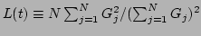
Since our simulation is of microcanonical ensemble, we have
monitored various statistics of the system to verify that the
thermal equilibrium state that is consistent with the Gibbs
distribution (canonical ensemble) has been reached. Moreover, we
verified that, for as small as 32 and up to as large as 1024,
the equilibrium distribution in the thermalized state in our
microcanonical ensemble simulation is consistent with the Gibbs
measure. We compared the renormalization factor (25) by
computing the values of
.
Since our simulation is of microcanonical ensemble, we have
monitored various statistics of the system to verify that the
thermal equilibrium state that is consistent with the Gibbs
distribution (canonical ensemble) has been reached. Moreover, we
verified that, for as small as 32 and up to as large as 1024,
the equilibrium distribution in the thermalized state in our
microcanonical ensemble simulation is consistent with the Gibbs
measure. We compared the renormalization factor (25) by
computing the values of
 and
and
 numerically and
theoretically using the Gibbs measure and found the discrepancy of
numerically and
theoretically using the Gibbs measure and found the discrepancy of
 to be within
  for
for  and the energy density
 for from 32 to 1024.
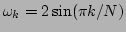
We now address numerically how the renormalized linear dispersion
manifests itself in the dynamics of the -FPU system.
We compute the spatiotemporal spectrum
 , where
 is the Fourier transform of
 . (Note that, for
simplicity of notation, we drop a tilde in
. (Note that, for
simplicity of notation, we drop a tilde in  .)
.)
Figure:
The spatiotemporal spectrum
in thermal
equilibrium. The chain was modeled for  ,
,  , and
, and
 . [
. [
 , with corresponding gray
scale, is plotted for a clear presentation]. The solid curve
corresponds to the usual linear dispersion
, with corresponding gray
scale, is plotted for a clear presentation]. The solid curve
corresponds to the usual linear dispersion
 .
The dashed curve shows the locations of the actual frequency peaks
of
.
.
The dashed curve shows the locations of the actual frequency peaks
of
.
![\includegraphics[width=3in, height=2.5in]{awk_num}](img148.png) |
Figure 1 displays the spatiotemporal spectrum of
, obtained from the simulation of the -FPU chain for
, , and . In order to measure the value of
from the spatiotemporal spectrum, we use the following
procedure. For the fixed wave number  , the corresponding
renormalization factor
, the corresponding
renormalization factor  is determined by the location of
the center of the frequency spectrum
, i.e.,
is determined by the location of
the center of the frequency spectrum
, i.e.,
 with with |
|
|
|
The
renormalization factor of each wave mode is shown in
Fig. 2 (inset). The numerical approximation
 to the value of is obtained by averaging all , i.e.,
The renormalization factor for the case shown in
Fig. 1 is measured to be
 .
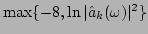
It can be clearly seen in Fig. 2 (inset) that
is nearly independent of and its variations around
are less than
.
It can be clearly seen in Fig. 2 (inset) that
is nearly independent of and its variations around
are less than  . We also compare the renormalization factor
obtained from Eq. (25) (solid line in
Fig. 2 (inset)) with its numerically computed
approximation
(dashed line in
Fig. 2 (inset)). Equation (25) gives the value
. We also compare the renormalization factor
obtained from Eq. (25) (solid line in
Fig. 2 (inset)) with its numerically computed
approximation
(dashed line in
Fig. 2 (inset)). Equation (25) gives the value
 and the difference between and
is less then , which can be attributed to the
statistical errors in the numerical measurement.
and the difference between and
is less then , which can be attributed to the
statistical errors in the numerical measurement.
Figure 2:
The renormalization factor as a function of the
nonlinearity strength . The analytical prediction
[Eq. (25)] is depicted with a solid line and the numerical
measurement is shown with circles. The chain was modeled for
, and . Inset: Independence of of the
renormalization factor . The circles correspond to
obtained from the spatiotemporal spectrum shown in
Fig. 1 [only even values of are shown for
clarity of presentation]. The dashed line corresponds to the mean
value
. For , the mean value of the
renormalization factor is found to be
. The
variations of  around
are less then .
[Note the scale of the ordinate.] The solid line corresponds to the
renormalization factor obtained from Eq. (25). For the
given parameters
.
around
are less then .
[Note the scale of the ordinate.] The solid line corresponds to the
renormalization factor obtained from Eq. (25). For the
given parameters
.
![\includegraphics[width=3in, height=2.5in]{etak_in}](img154.png) |
In Fig. 2, we plot the value of as a function of
for the system with particles and the total energy
. The solid curve was obtained using Eq. (25) while
the circles correspond to the value of determined via the
numerical spectrum
as discussed above. It can be
observed that there is excellent agreement between the theoretic
prediction and numerically measured values for a wide range of the
nonlinearity strength .
In the following Sections, we will discuss how the renormalization
of the linear dispersion of the -FPU chain in thermal
equilibrium can be explained from the wave resonance point of view.
In order to give a wave description of the -FPU chain, we
rewrite the Hamiltonian (29) in terms of the renormalized
variables
[Eq. (19)] with
 ,
,
where c.c. stands for complex conjugate, and
 |
|
|
(33) |
is the interaction tensor coefficient. Note that, due to the
discrete nature of the system of finite size, the wave space is
periodic and, therefore, the ``momentum'' conservation is guaranteed
by the following ``periodic'' Kronecker delta functions
Here, the Kronecker  -function is equal to 1, if the sum
of all superscripts is equal to the sum of all subscripts, and 0,
otherwise.
-function is equal to 1, if the sum
of all superscripts is equal to the sum of all subscripts, and 0,
otherwise.
Next: Dispersion relation and resonances
Up: Interactions of renormalized waves
Previous: Renormalized waves
Dr Yuri V Lvov
2007-04-11
![$\displaystyle \frac{1}{2}p_j^2+\frac{1}{4}\big[(q_j-q_{j+1})^2+(q_{j-1}-q_j)^2\big]$](img134.png)
![$\displaystyle \frac{\beta}{8}\big[(q_j-q_{j+1})^4+(q_{j-1}-q_j)^4\big].$](img135.png)

![$\displaystyle \left(\frac{1}{6}\Delta ^{klms}_{0}\tilde{a}_k\tilde{a}_l\tilde{a}_m\tilde{a}_s+c.c.\right)\Big],$](img160.png)