Dispersion relation and resonances

In order to address how the renormalized dispersion arises from wave interactions, we study the resonance structure of our nonlinear waves. Since the system (32) is a Hamiltonian system with four-wave interactions, we will discuss the properties of the resonance manifold associated with the $\beta$-FPU system described by Eq. (32) as a first step towards the understanding of its long time statistical behavior. We comment that the resonance structure is one of the main objects of investigation in wave turbulence theory [5,22,23,24,25,26,27]. The theory of wave turbulence focuses on the specific type of interactions, namely resonant interactions, which dominate long time statistical properties of the system. On the other hand, the non-resonant interactions are usually shown to have a total vanishing average contribution to a long time dynamics.

In analogy with quantum mechanics, where $a^+$ and $a$ are creation and annihilation operators, we can view $\tilde{a}_k^*$ as the outgoing wave with frequency $\tilde{\omega}_k$ and $\tilde{a}_k$ as the incoming wave with frequency $\tilde{\omega}_k$. Then, the nonlinear term $\tilde{a}_k^*\tilde{a}_l^*\tilde{a}_m\tilde{a}_s\Delta^{kl}_{ms}$ in system (32) can be interpreted as the interaction process of the type $(2\rightarrow 2)$, namely, two outgoing waves with wave numbers $k$ and $l$ are ``created'' as a result of interaction of the two incoming waves with wave numbers $m$ and $s$. Similarly, $\tilde{a}_k^*\tilde{a}_l\tilde{a}_m\tilde{a}_s\Delta_{k}^{lms}$ in system (32) describes the interaction process of the type $(3\rightarrow 1)$, that is, one outgoing wave with wave number $k$ is ``created'' as a result of interaction of the three incoming waves with wave numbers $l$, $m$, and $s$, respectively. Finally, $\tilde{a}_k\tilde{a}_l\tilde{a}_m\tilde{a}_s\Delta_{0}^{klms}$ describes the interaction process of the type $(4\rightarrow 0)$, i.e., all four incoming waves interact and annihilate themselves. Furthermore, the complex conjugate terms $\tilde{a}_k\tilde{a}_l^*\tilde{a}_m^*\tilde{a}_s^*\Delta_{lms}^{k}$ and $\tilde{a}_k^*\tilde{a}_l^*\tilde{a}_m^*\tilde{a}_s^*\Delta^{0}_{klms}$ describe the interaction processes of the type $(1\rightarrow 3)$ and $(0\rightarrow 4)$, respectively.

Instead of the processes with the ``momentum'' conservation given via the usual $\delta^{kl}_{ms}$, $\delta^{klm}_s$, or $\delta^{klms}_0$ functions for an infinite discrete system, the resonant processes of the $\beta$-FPU chain of a finite size are constrained to the manifold given by $\Delta ^{kl}_{ms}$, $\Delta ^{klm}_s$, or $\Delta ^{klms}_0$, respectively. Next, we describe these resonant manifolds in detail. As will be pointed out in Section VI, there is a consequence of this finite size effect to the properties of the renormalized waves.

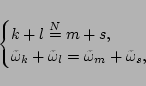
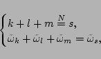
The resonance manifold that corresponds to the $(2\rightarrow 2)$ resonant processes in the discrete periodic system, therefore, is described by

$$\begin{cases} k+l\overset{N}{=}m+s,\\ \tilde{\omega}_k+\tilde{\omega}_l=\tilde{\omega}_m+\tilde{\omega}_s, \end{cases}$$ (37)

where we have introduced the notation $g\overset{N}{=}h$, which means that $g=h$, $g=h+N$, or $g=h-N$ for any $g$ and $h$. The first equation in system (37) is the ``momentum'' conservation condition in the periodic wave number space. This ``momentum'' conservation comes from $\vert\Delta ^{kl}_{ms}\vert=1$. 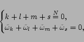(Note that $\vert\Delta ^{kl}_{ms}\vert$ can assume only the value of $1$ or 0.) Similarly, from $\vert\Delta ^{klm}_{s}\vert=1$ and $\vert\Delta ^{klms}_{0}\vert=1$, the resonance manifolds corresponding to the resonant processes of types $(3\rightarrow 1)$ and $(4\rightarrow 0)$ are given by

$$\begin{cases} k+l+m\overset{N}{=}s,\\ \tilde{\omega}_k+\tilde{\omega}_l+\tilde{\omega}_m=\tilde{\omega}_s, \end{cases}$$ (38)

and

$$\begin{cases} k+l+m+s\overset{N}{=}0,\\ \tilde{\omega}_k+\tilde{\omega}_l+\tilde{\omega}_m+\tilde{\omega}_s=0, \end{cases}$$ (39)

respectively. For the processes of type $(3\rightarrow 1)$, the notation $g\overset{N}{=}h$ means that $g=h$, $g=h+N$, or $g=h+2N$. For the $(4\rightarrow 0)$ processes, $g\overset{N}{=}h$ means that $g=h+N$, $g=h+2N$, or $g=h+3N$.

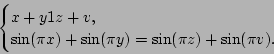
To solve system (37), we rewrite it in a continuous form with $x={k}/{N}$, $y={l}/{N}$, $z={m}/{N}$, $v={s}/{N}$, which are real numbers in the interval $(0,1)$. By recalling that $\tilde{\omega}_k=2\eta\sin({\pi k}/{N})$, we have

$$\begin{cases} x+y\eq1 z+v,\\ \sin(\pi x)+\sin(\pi y)=\sin(\pi z)+\sin(\pi v). \end{cases}$$ (40)

Thus, any rational quartet that satisfies Eq. (40) yields a solution for Eq. (37). There are two distinct types of the solutions of Eq. (40). The first one corresponds to the case

$$x+y=z+v,$$

whose only solution is given by

$$\begin{cases} x=z,\\ y=v, \end{cases}\mbox{or}~~ \begin{cases} x=v,\\ y=z,\end{cases}$$ (41)

i.e., these are trivial resonances, as we mentioned above. The second type of the resonance manifold of the $(2\rightarrow 2)$-type interaction processes corresponds to

$$x+y=z+v\pm 1,$$

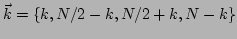
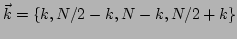
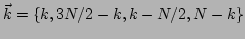
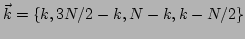
the solution of which can be described by the following two branches

$$z_1 = \frac{x+y}{2}+\frac{1}{\pi}\arcsin(A)+2j,$$ (42)

$$z_2 = \frac{x+y}{2}-1-\frac{1}{\pi}\arcsin(A)+2j,$$ (43)

where $A\equiv\tan\left(\pi({x+y})/{2}\right)\cos\left(\pi({x-y})/{2}\right)$ and $j$ is an integer. The second type of resonances arises from the discreteness of our model of a finite length, leading to non-trivial resonances. For our linear dispersion here, non-trivial resonances are only those resonances that involve wave numbers crossing the first Brillouin zone. As mentioned above, in the setting of the phonon physics, these non-trivial resonant processes are also known as the umklapp scattering processes. In Fig. 3, we plot the solution of Eq. (40) for $x={k}/{N}$ with the wave number $k=90$ for the system with $N=256$ particles (the values of $k$ and $N$ are chosen merely for the purpose of illustration). We stress that all the solutions of the system (40) are given by the Eqs. (41), (42), and (43), and that the non-trivial solutions arise only as a consequence of discreteness of the finite chain. The curves in Fig. 3 represent the loci of $(z,y)$, parametrized by the fourth wave number $v$, i.e., $x$, $y$, $z$, and $v$ form a resonant quartet, where $z={m}/{N}$, and $y={l}/{N}$. Note that the fourth wave number $v$ is specified by the ``momentum'' conservation, i.e., the first equation in Eq. (40). The two straight lines in Fig. 3 correspond to the trivial solutions, as given by Eq. (41). The two curves (dotted and dashed) depict the non-trivial resonances. Note that the dotted part of non-trivial resonance curves corresponds to the branch (42), and the dashed part corresponds to the branch (43), respectively. An immediate question arises: how do these resonant structures manifest themselves in the FPU dynamics in the thermal equilibrium? By examining the Hamiltonian (32), we notice that the resonance will control the contribution of terms like $\tilde{a}_k^*\tilde{a}_l^*\tilde{a}_m\tilde{a}_s\Delta^{kl}_{ms}$ in the long time limit. Therefore, we address the effect of resonance by computing long time average, i.e., $\langle \tilde{a}_k^*\tilde{a}_l^*\tilde{a}_m\tilde{a}_s\rangle \Delta ^{kl}_{ms}$, and comparing this average (Fig. 4) with Fig. 3.

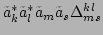
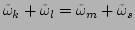
Figure 3: The solutions of Eq. (40). The solid straight lines correspond to the trivial resonances [solutions of Eq. (41)]. The solutions are shown for fixed $x=k/N$, $k=90$, $N=256$ as the fourth wave number $v$ scans from ${1}/{N}$ to $(N-1)/{N}$ in the resonant quartet Eq. (40). The non-trivial resonances are described by the dotted or dashed curves. The dotted branch of the curves corresponds to the non-trivial resonances described by Eq. (42) and and the dashed branch corresponds to the non-trivial resonances described by Eq. (43).

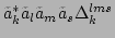
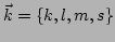
Figure: The long time average $\vert\langle \tilde{a}_k^*\tilde{a}_l^*\tilde{a}_m\tilde{a}_s\rangle \Delta ^{kl}_{ms}\vert$ of the $\beta$-FPU system in thermal equilibrium. The parameters for the FPU chain are $N=256$, $\beta =0.5$, and $E=100$. $\langle \tilde{a}_k^*\tilde{a}_l^*\tilde{a}_m\tilde{a}_s\rangle \Delta ^{kl}_{ms}$ was computed for fixed $k=90$. The darker grayscale corresponds to the larger value of $\langle \tilde{a}_k^*\tilde{a}_l^*\tilde{a}_m\tilde{a}_s\rangle \Delta ^{kl}_{ms}$. The exact solutions of Eq. (40), which are shown in Fig. 3, coincide with the locations of the peaks of $\vert\langle \tilde{a}_k^*\tilde{a}_l^*\tilde{a}_m\tilde{a}_s\rangle \Delta ^{kl}_{ms}\vert$. Therefore, the darker areas represent the near-resonance structure of the finite $\beta$-FPU chain. (The two white lines show the locations, where $s=0$ and, therefore, $\tilde{a}_k^*\tilde{a}_l^*\tilde{a}_m\tilde{a}_s\Delta ^{kl}_{ms}=0$.) [ $\max\{2,\ln(\vert\langle \tilde{a}_k^*\tilde{a}_l^*\tilde{a}_m\tilde{a}_s\rangle \Delta ^{kl}_{ms}\vert)\}$ with the corresponding grayscale is plotted for a clean presentation].

To obtain Fig. 4, the $\beta$-FPU system was simulated with the following parameters: $N=256$, $\beta =0.5$, $E=100$, and the averaging time window $\tau=400\tilde{t}_1$, where $\tilde{t}_1$ is the longest linear period, i.e., $\tilde{t}_1={2\pi}/{\tilde{\omega}_1}$. In Fig. 4, mode $k$ was fixed with $k=90$ and the mode $s$, a function of $k$, $l$, and $m$, is obtained from the constraint $k+l\overset{N}{=}m+s$, i.e., $\vert\Delta ^{kl}_{ms}\vert=1$. Note that we do not impose here the condition $\tilde{\omega}_k+\tilde{\omega}_l=\tilde{\omega}_m+\tilde{\omega}_s$, therefore, $\vert\langle \tilde{a}_k^*\tilde{a}_l^*\tilde{a}_m\tilde{a}_s\rangle \Delta ^{kl}_{ms}\vert$ is a function of $l$ and $m$. By comparing Figs. 3 and 4, it can be observed that the locations of the peaks of the long time average $\vert\langle \tilde{a}_k^*\tilde{a}_l^*\tilde{a}_m\tilde{a}_s\rangle \Delta ^{kl}_{ms}\vert$ coincide with the loci of the $(2\rightarrow 2)$-type resonances. This observation demonstrates that, indeed, there are nontrivial $(2\rightarrow 2)$-type resonances in the finite $\beta$-FPU chain in thermal equilibrium. Furthermore, it can be observed in Fig. 4 that, in addition to the fact that the resonances manifest themselves as the locations of the peaks of $\vert\langle \tilde{a}_k^*\tilde{a}_l^*\tilde{a}_m\tilde{a}_s\rangle \Delta ^{kl}_{ms}\vert$, the structure of near-resonances is reflected in the finite width of the peaks around the loci of the exact resonances. Note that, due to the discrete nature of the finite $\beta$-FPU system, only those solutions $x$, $y$, $z$, and $v$ of Eq. (40), for which $Nx$, $Ny$, $Nz$, and $Nv$ are integers, yield solutions $k$, $l$, $m$, and $s$ for Eq. (37). In general, the rigorous treatment of the exact integer solutions of Eq. (37) is not straightforward. For example, for $N=256$, we have the following two exact quartets $\vec{k}=\{k,l,m,s\}$: $\vec{k}=\{k,N/2-k,N/2+k,N-k\}$, $\vec{k}=\{k,N/2-k,N-k,N/2+k\}$ for $k<N/2$, and $\vec{k}=\{k,3N/2-k,k-N/2,N-k\}$, $\vec{k}=\{k,3N/2-k,N-k,k-N/2\}$ for $k>N/2$. We have verified numerically that for $N=256$ there are no other exact integer solutions of Eq. (37). In the analysis of the resonance width in Section VI, we will use the fact that the number of exact non-trivial resonances [Eq. (37)] is significantly smaller than the total number of modes.

The broadening of the resonance peaks in Fig. 4 suggests that, to capture the near-resonances for characterizing long time statistical behavior of the $\beta$-FPU system in thermal equilibrium, instead of Eq. (37), one needs to consider the following effective system

$$\begin{cases} k+l\overset{N}{=}m+s,\\ \vert\tilde{\omega}_k+... ...ilde{\omega}_m-\tilde{\omega}_s\vert<\Delta\omega , \end{cases}$$ (44)

where $0<\Delta\omega \ll\tilde{\omega}_k$ for any $k$, and $\Delta\omega$ characterizes the resonance width, which results from the near-resonace structure. Clearly, $\Delta\omega$ is related to the broadening of the spectral peak of each wave $\tilde{a}_{\alpha }(t)$ with $\alpha =k,l,m$, or $s$ in the quartet, and this broadening effect will be studied in detail in Section VI. Note that the structure of near-resonances is a common characteristic of many periodic discrete nonlinear wave systems [28,29,30].

Further, it is easy to show that the dispersion relation of the $\beta$-FPU chain does not allow for the occurrence of $(3\rightarrow 1)$-type resonances, i.e., there are no solutions for Eq. (38), and, therefore, all the nonlinear terms $\tilde{a}_k^*\tilde{a}_l\tilde{a}_m\tilde{a}_s\Delta ^{k}_{lms}$ are non-resonant and their long time average $\langle \tilde{a}_k^*\tilde{a}_l\tilde{a}_m\tilde{a}_s\rangle \Delta ^{k}_{lms}$ vanishes. As for the resonances of type $(4\rightarrow 0)$, since the dispersion relation is non-negative, one can immediately conclude that the solution of the system (39) consists only of zero modes. Therefore, the processes of type $(4\rightarrow 0)$ are also non-resonant, giving rise to $\langle \tilde{a}_k\tilde{a}_l\tilde{a}_m\tilde{a}_s\rangle \Delta _{0}^{klms}=0$. In this article, we will neglect the higher order effects of the near-resonances of the types $(3\rightarrow 1)$ and $(4\rightarrow 0)$.

In the following sections, we will study the effects of the resonant terms of type $(2\rightarrow 2)$, namely, the linear dispersion renormalization and the broadening of the frequency peaks of $\tilde{a}_k(t)$. It turns out that, the former is related to the trivial resonance of type $(2\rightarrow 2)$ and the latter is related to the near-resonances, as will be seen below.