Resonance width

Finally, we address the question of how coherent these renormalized waves are, i.e., we study how the nonlinear interactions of waves in thermal equilibrium broaden the renormalized dispersion. We will obtain an analytical formula for the spatiotemporal spectrum $\vert\hat{a}_k(\omega )\vert^2$ for the $\beta$-FPU chain and compare the numerically measured width of the frequency peaks with the predicted width.

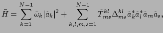
In the Hamiltonian (46), the nonlinear terms corresponding to the trivial resonances have been absorbed into the quadratic part via the effective renormalized dispersion $\tilde{\omega}_k$. Therefore, the new effective Hamiltonian is

$$\bar{H}=\sum_{k=1}^{N-1}\tilde{\omega}_k\vert\tilde{a}_k\vert^2+\... ...e{T}^{kl}_{ms}\Delta^{kl}_{ms}\tilde{a}_k^*\tilde{a}_l^*\tilde{a}_m\tilde{a}_s,$$ (54)

where

$$\begin{cases} \tilde{T}^{kl}_{ms}=T^{kl}_{ms}=\displaystyle{\... ...\neq s\\ \tilde{T}^{kl}_{ms}=0,~~\mbox{otherwise.} \end{cases}$$ (55)

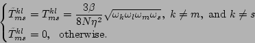
The new interaction coefficient $\tilde{T}^{kl}_{ms}$ ensures that the terms that correspond to the interactions with trivial resonances are not doubly counted in the Hamiltonian (55) and are removed from the quartic interaction. This new interactions in the quartic terms include the exact non-trivial resonant and non-trivial near-resonant as well as non-resonant interactions of the $(2\rightarrow 2)$-type.

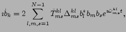
We change the variables to the interaction picture by defining the corresponding variables $b_k$ via

$$b_k=\tilde{a}_ke^{\imath \tilde{\omega}_kt},$$

so that, the dynamics governed by the Hamiltonian (55) takes the familiar form

$$\imath \dot b_k=2\sum_{l,m,s=1}^{N-1}\tilde{T}^{kl}_{ms}\Delta^{kl}_{ms}b_l^*b_mb_se^{\imath \tilde{\omega}^{kl}_{ms} t},$$ (56)

where $\tilde{\omega}^{kl}_{ms}=\tilde{\omega}_k+\tilde{\omega}_l-\tilde{\omega}_m-\tilde{\omega}_s$ [23]. Without loss of generality, we consider only the case of $k<N/2$. As we have noted before, only for a very small number of quartets does $\tilde{\omega}^{kl}_{ms}$ vanish exactly, i.e., $\tilde{\omega}^{kl}_{ms}=0$. We separate the terms on the RHS of Eq. (57) into two kinds -- the first kind with $\tilde{\omega}^{kl}_{ms}=0$ that corresponds to exact non-trivial resonances, and the second kind that corresponds to non-trivial near-resonances and non-resonances. Since, in the summation, the first kind contains far fewer terms than the second kind, and all the terms are of the same order of magnitude, we will neglect the first kind in our analysis. Therefore, Eq. (57) becomes

$$\imath \dot b_k = 2{\sum_{l,m,s=1}^{N-1}}^{\prime} \tilde{T}^{kl}_{ms}\Delta^{kl}_{ms}b_l^*b_mb_se^{\imath \tilde{\omega}^{kl}_{ms} t},$$ (57)

where the prime denotes the summation that neglects the exact non-trivial resonances.

The problem of broadening of spectral peaks now becomes the study of the frequency spectrum of the dynamical variables $b_k(t)$ in thermal equilibrium. This is equivalent to study the two-point correlation in time of $b_k(t)$

$$C_k(t)=\langle b_k(t)b_k^*(0)\rangle ,$$ (58)

where the angular brackets denote the thermal average, since, by Wiener-Khinchin theorem, the frequency spectrum

$$\vert b(\omega )\vert^2=\mathfrak{F}^{-1}[C(t)](\omega ),$$ (59)

where $\mathfrak{F}^{-1}$ is the inverse Fourier transform in time. Under the dynamics (58), time derivative of the two-point correlation becomes

$$\dot{C}_k(t) = \langle \dot{b}_k(t)b_k^*(0)\rangle$$

$$= \langle -2\imath {\sum_{l,m,s}}^{\prime}\tilde{T}^{kl}_{ms}b_l^*(t)b_m(t)b_s(t)e^{\imath \tilde{\omega}^{kl}_{ms}t}\Delta^{kl}_{ms}b_k^*(0)\rangle$$

$$= -2\imath {\sum_{l,m,s}}^{\prime}\tilde{T}^{kl}_{ms}e^{\imath \tilde{\omega}^{kl}_{ms}t}J^{kl}_{ms}(t)\Delta^{kl}_{ms},$$ (60)

where

$$J^{kl}_{ms}(t)\equiv\langle b_l^*(t)b_k^*(0)b_m(t)b_s(t)\rangle .$$

In order to obtain a closed equation for $C_k(t)$, we need to study the evolution of the fourth order correlator $J^{kl}_{ms}(t)$. We utilize the weak effective nonlinearity in Eq. (55) [12] as the small parameter in the following perturbation analysis and obtain a closure for $C_k(t)$, similar to the traditional way of deriving kinetic equation, as in [5,31]. We note that the effective interactions of renormalized waves can be weak, as we have shown in [12], even if the $\beta$-FPU chain is in a strongly nonlinear regime. Our perturbation analysis is a multiple time-scale, statistical averaging method. Under the near-Gaussian assumption, which is applicable for the weakly nonlinear wave fields in thermal equilibrium, for the four-point correlator, we obtain

$$J^{kl}_{ms}(t)\Delta^{kl}_{ms}=C_k(t)C_l(0)(\delta^k_m\delta^l_s+\delta^k_s\delta^l_m).~~$$ (61)

Combining Eqs. (56) and (62), we find that the right-hand side of Eq. (61) vanishes because

$$\tilde{T}^{kl}_{ms}J^{kl}_{ms}(t)\Delta^{kl}_{ms}=0.$$ (62)

Therefore, we need to proceed to the higher order contribution of $J^{kl}_{ms}(t)$. Taking its time derivative yields

$$\dot{J}^{kl}_{ms}(t)\Delta ^{kl}_{ms} = \langle [\dot{b}_l^*(t)b_m(t)b_s(t)+b_l^*(t)\dot{b}_m(t)b_s(t)$$

$$+ b_l^*(t)b_m(t)\dot{b}_s(t)]b_k^*(0)\rangle \Delta ^{kl}_{ms}.$$ (63)

Considering the right-hand side of Eq. (64) term by term, for the first term, we have

$$\langle \dot{b}_l^*(t)b_m(t)b_s(t)b_k^*(0)\rangle \Delta ^{kl}_{ms}$$

$$=\Bigg\langle \Big[2\imath {\sum_{\alpha ,\beta ,\gamma }}^{\prim... ...ilde{T}^{l\alpha }_{\beta \gamma }b_{\alpha }(t)b_{\beta }^*(t)b_{\gamma }^*(t)$$

$$\times e^{-\imath \omega ^{l\alpha }_{\beta \gamma }}\Delta ^{l\alpha }_{\beta \gamma }\Big]b_m(t)b_s(t)b_k^*(0)\Bigg\rangle \Delta ^{kl}_{ms}.$$ (64)

We can use the near-Gaussian assumption to split the correlator of the sixth order in Eq. (65) into the product of three correlators of the second order, namely,

$$\langle b_k^*(0)b_m(t)b_s(t)b_{\alpha }(t)b_{\beta }^*(t)b_{\gamma }^*\rangle \Delta ^{kl}_{ms}$$

$$=C_k(t)n_m n_s\delta^k_{\alpha }(\delta_{\beta }^m\delta^s_{\gamma }+\delta^m_{\gamma }\delta^s_{\beta }),$$

where we have used that $n_m=C_m(0)$. Then, Eq. (65) becomes

$$\langle \dot{b}_l^*(t)b_m(t)b_s(t)b_k^*(0)\rangle \Delta ^{kl}_{ms}$$

$$=4\imath \tilde{T}^{lk}_{ms}C_k(t)n_m n_s e^{-\imath \tilde{\omega}^{lk}_{ms}}\Delta ^{kl}_{ms}.$$ (65)

Similarly, for the remaining two terms in Eq. (64), we have

$$\langle b_l^*(t)\dot{b}_m(t)b_s(t)b_k^*(0)\rangle \Delta ^{kl}_{ms}$$

$$=-4\imath \tilde{T}^{ms}_{kl}C_k(t)n_l n_s e^{\imath \tilde{\omega}^{ms}_{kl}}\Delta ^{kl}_{ms},$$ (66)

and

$$\langle b_l^*(t)b_m(t)\dot{b}_s(t)b_k^*(0)\rangle \Delta ^{kl}_{ms}$$

$$=-4\imath \tilde{T}^{ms}_{kl}C_k(t)n_l n_m e^{\imath \tilde{\omega}^{ms}_{kl}}\Delta ^{kl}_{ms},$$ (67)

respectively. Combining Eqs. (66), (67), and (68) with Eq. (64), we obtain

$$\dot{J}^{kl}_{ms}(t)\Delta ^{kl}_{ms} = 4\imath \tilde{T}^{kl}_{ms}C_k(t)e^{-\imath \tilde{\omega}^{kl}_{ms}t}\Delta ^{kl}_{ms}$$

$$\times(n_m n_s-n_l n_m-n_l n_s).$$ (68)

Equation (69) can be solved for $J^{kl}_{ms}(t)$ under the assumption that the term $e^{-\imath \tilde{\omega}^{kl}_{ms}t}$ oscillates much faster than $C_k(t)$. We numerically verify [Fig. 9 below] the validity of this assumption of time-scale separation. Under this approximation, the solution of Eq. (69) becomes

$$J^{kl}_{ms}(t)\Delta ^{kl}_{ms} = 4\tilde{T}^{kl}_{ms}C_k(t)\Delta ^{kl}_{ms}\frac{e^{-\imath \tilde{\omega}^{kl}_{ms}t}-1}{-\tilde{\omega}^{kl}_{ms}}$$

$$\times(n_m n_s-n_l n_m-n_l n_s )$$ (69)

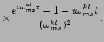
Plugging Eq. (70) into Eq. (61), we obtain the following equation for $C_k(t)$

$$\dot{C}_k(t) = 8\imath C_k(t) {\sum_{l,m,s}}^{\prime} \left(\tilde{T}^{kl}_{ms}\right)^2\Delta ^{kl}_{ms}\frac{1-e^{\imath \omega ^{kl}_{ms}t}}{\omega ^{kl}_{ms}}$$

$$\times(n_m n_s-n_l n_s-n_l n_m).$$ (70)

Since in the thermal equilibrium $n_k$ is known, i.e., $n_k=\langle \vert b_k(t)\vert^2\rangle =\theta/\tilde{\omega}_k$ [Eq. (26)], Eq. (71) becomes a closed equation for $C_k(t)$. The solution of Eq. (71) yields the autocorrelation function $C_k(t)$

$$\ln\frac{C_k(t)}{C_k(0)} = 8{\sum_{l,m,s}}^{\prime} \left(\tilde{T}^{kl}_{ms}\right)^2\frac{e^{\imath \omega ^{kl}_{ms}t}-1-\imath \omega ^{kl}_{ms}t}{(\omega ^{kl}_{ms})^2}$$

$$\times(n_l n_s+n_l n_m-n_m n_s)\Delta ^{kl}_{ms}.$$ (71)

Using this observation, together with Eq. (56), finally, we obtain for the thermalized $\beta$-FPU chain

$$\ln\frac{C_k(t)}{C_k(0)} = \frac{9\beta^2\theta^2}{8N^2\eta^6}\omega _k{\sum_{l,m,s}}^{\prime}(\omega _m+\omega _s-\omega _l)\Delta ^{kl}_{ms}$$

$$\times\frac{e^{\imath \omega ^{kl}_{ms}t}-1-\imath \omega ^{kl}_{ms}t}{(\omega ^{kl}_{ms})^2}.$$ (72)

Equation (73) gives a direct way of computing the correlation function of the renormalized waves $\tilde{a}_k$, which, in turn, allows us to predict the spatiotemporal spectrum $\vert\hat{a}_k(\omega )\vert^2$. In Fig. 6(a), we plot the analytical prediction (via Eq. (73)) of the spatiotemporal spectrum $\vert\hat{a}_k(\omega )\vert^2\equiv\vert b_k(\omega -\tilde{\omega}_k)\vert^2=\mathfrak{F}^{-1}[C(t)](\omega -\tilde{\omega}_k)$. By comparing this plot with the one presented in Fig. 6(b), in which the corresponding numerically measured spatiotemporal spectrum is shown, it can be seen that the analytical prediction of the frequency spectrum via Eq. (73) is in good qualitative agreement with the numerically measured one. However, to obtain a more detailed comparison of the analytical prediction with the numerical observation, we show, in Fig. 7, the numerical frequency spectra of selected wave modes with the corresponding analytical predictions. It can be clearly observed that the agreement is rather good.

Figure: (a) Plot of the analytical prediction for the spatiotemporal spectrum $\vert\hat{a}_k(\omega )\vert^2$ via Eq. (73). (b) Plot of the numerically measured spatiotemporal spectrum $\vert\hat{a}_k(\omega )\vert^2$. The parameters in both plots were $N=256$, $\beta =0.125$, $E=100$ and $\eta =1.06$, $\theta =0.401$. $\eta$ and $\theta$ were computed analytically via Gibbs measure. The darker gray scale correspond to larger values of $\vert\hat{a}_k(\omega )\vert^2$ in $\omega$-$k$ space. [ $\max\{-8,\ln{\vert\hat{a}_k(\omega )\vert^2}\}$ is plotted for clear presentation].

Figure: Temporal frequency spectrum $\vert\hat{a}_k(\omega )\vert^2$ for $k=30$ (left peak) and $k=50$ (right peak). The numerical spectrum is shown with pluses and the analytical prediction [via Eq. (73)] is shown with solid line. The parameters were $N=256$, $\beta =0.125$, $E=100$.

One of the important characteristics of the frequency spectrum is the width of the spectrum. We compute the width $W(f)$ of the spectrum $f(\omega )$ by

$$W(f)=\frac{\int f(\omega )~d\omega }{\max_\omega f(\omega )}.$$ (73)

In Fig. 8, we compare the width, as a function of the wave number $k$, of the frequency peaks from the numerical observation with that obtained from the analytical predictions. We observe that, for weak nonlinearity ( $\beta =0.125$), the analytical prediction and the numerical observation are in excellent agreement. In the weakly nonlinear regime, this agreement can be attributed to the validity of (i) the near-Gaussian assumption, and (ii) the separation between the linear dispersion time scale and the time scale of the correlation $C_k(t)$. This separation was used in deriving the analytical prediction [Eq. (73)]. However, when the nonlinearity becomes larger ( $\beta =0.25$ and $\beta =0.5$), the discrepancy between the numerical measurements and the analytical prediction increases, as can be seen in Fig. 8. Nevertheless, it is important to emphasize that, even for very strong nonlinearity, our prediction is still qualitatively valid, as seen in Fig. 8. In order to find out the effect of the umklapp scattering due to the finite size of the chain, we also computed the correlation [Eq. (73)] with the ``conventional'' $\delta$-function $\delta^{kl}_{ms}$ (i.e., without taking into account the umklapp processes) instead of our ``periodic'' delta function $\Delta ^{kl}_{ms}$. It turns out that the correlation time is approximately $30\%$ larger if it is computed without umklapp processes taken into account for the case $N=256$, $\beta =0.5$, $E=100$. It demonstrates that the influence of the non-trivial umklapp resonances is important and should be considered when one describes the dynamics of the finite length chain of particles.

Figure: Frequency peak width $W(\vert\hat{a}_k(\omega )\vert^2)$ as a function of the wave number $k$. The analytical prediction via Eq. (73) is shown with a dashed line and the numerical observation is plotted with solid circles. The parameters were $N=256$, $E=100$. The upper thick lines correspond to $\beta =0.5$, the middle fine lines correspond to $\beta =0.25$, and the lower solid circle and dashed line (almost overlap) correspond to $\beta =0.125$.

Finally, in Fig. 9, we verify the time scale separation assumption used in our derivation, i.e., the correlation time of the wave mode $k$ is sufficiently larger than the corresponding linear dispersion period $\tilde{t}_k=2\pi/\tilde{\omega}_k$. In the case of small nonlinearity ( $\beta =0.125$), the two-point correlation changes over much slower time scale than the corresponding linear oscillations -- the correlation time is nearly two orders of magnitude larger than the corresponding linear oscillations for weak nonlinearity $\beta =0.125$, and nearly one order of magnitude larger than the corresponding linear oscillations for stronger nonlinearity $\beta =0.25$ and $\beta =0.5$. This demonstrates that the renormalized waves have long lifetimes, i.e., they are coherent over time-scales that are much longer than their oscillation time-scales.

Figure 9: Ratio, as a function of $k$, of the correlation time $\tau _k$ of the mode $k$ to the corresponding linear period $\tilde{t}_k=2\pi/\tilde{\omega}_k$. Circles, squares, and diamonds represent the analytical prediction for $\beta =0.5$, $\beta =0.25$, and $\beta =0.125$ respectively. Stars, pentagrams, and triangles correspond to the numerical observation for $\beta =0.5$, $\beta =0.25$, and $\beta =0.125$ respectively. The parameters were $N=256$, $E=100$. The ratio is sufficiently large for all wave numbers $k$ even for relatively large $\beta =0.5$, which validates the time-scale separation assumption used in deriving Eq. (70). The comparison also suggests that for smaller $\beta$ the analytical prediction should be closer to the numerical observation, as is confirmed in Fig. 8.