Renormalized waves

Consider a chain of particles coupled via nonlinear springs. Suppose the total number of particles is $N$ and the momentum and displacement from the equilibrium position of the $j$-th particle are $p_j$ and $q_j$, respectively. If only the nearest-neighbor interactions are present, then the chain can be described by the Hamiltonian

$$H=H_2+V,$$ (6)

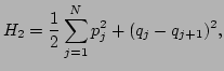
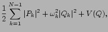
where the quadratic part of the Hamiltonian takes the form

$$H_2=\frac{1}{2}\sum_{j=1}^N{p_j^2}+(q_j-q_{j+1})^2,$$ (7)

and the anharmonic potential $V$ is the function of the relative displacement $q_j-q_{j+1}$. Here periodic boundary conditions $q_{N+1}\equiv q_1$ and $p_{N+1}\equiv p_1$ are imposed. Since the total momentum of the system is conserved, it can be set to zero.

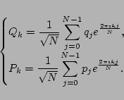
In order to study the distribution of energy among the wave modes, we transform the Hamiltonian to the Fourier variables $Q_k$, $P_k$ via

$$\begin{cases} Q_k=\displaystyle{\frac{1}{\sqrt{N}}}\sum_{j=0}... ...}}}\sum_{j=0}^{N-1}p_je^{\frac{2\pi \imath kj}{N}}. \end{cases}$$ (8)

This transformation is canonical [10,11] and the Hamiltonian (6) becomes

$$H = \frac{1}{2}\sum_{k=1}^{N-1}\vert P_k\vert^2+\omega_k^2\vert Q_k\vert^2+V(Q),$$ (9)

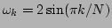where $\omega _k=2\sin(\pi k/N)$ is the linear dispersion relation. Note that, throughout the paper, for the simplicity of notation, we denote the periodic wave number space by the set of integers in the range $[0,N-1]$, i.e., we drop the conventional factor, $2\pi/N$. The zeroth mode vanishes due to the fact that the total momentum is zero.

If the system (9) is in thermal equilibrium, then the canonical Gibbs measure, with the corresponding partition function

$$Z=\int_{-\infty}^{\infty}e^{-H(p,q)/\theta}dpdq,$$ (10)

with the temperature $\theta$, can be used to describe the statistical behavior of the system. We consider the systems with the anharmonic potential of the restoring type, i.e., the potential for which the integral in Eq. (10) converges. It can be easily shown that for system (9) the average kinetic energy $K_k$ of each mode is independent of the wave number

$$\langle K_k\rangle =\langle K_l\rangle ,$$ (11)

where $k$ and $l$ are wave numbers, $K_k\equiv\vert P_k\vert^2/2$, and $\langle \dots\rangle$ denotes averaging over the Gibbs measure. Similarly, the average quadratic potential $U_k$ of each mode is independent of the wave number

$$\langle U_k\rangle =\langle U_l\rangle ,$$ (12)

where $U_k\equiv\omega _k^2\vert Q_k\vert^2/2$.

If the nonlinear interactions are weak, then it is convenient to further transform the Hamiltonian (9) to the complex normal variables defined by Eq. (2). This transformation is canonical, i.e., the dynamical equation of motion becomes

$$\imath \dot{a}_k=\frac{\partial H}{\partial a_k^*}.$$ (13)

In terms of these normal variables, the Hamiltonian (9) takes the form (3). For the system of noninteracting waves, i.e., $H=\sum_{k=1}^{N-1}\omega _k\vert a_k\vert^2$, we obtain a standard virial theorem in the form

$$\langle K_k\rangle \vline_{V=0}=\langle U_k\rangle \vline_{V=0}.$$ (14)

As a consequence of this virial theorem, we have the properties of free waves, which were already mentioned above [Eqs. (4) and (5)], i.e.,

$$\langle a_k^*a_l\rangle = \frac{1}{2\omega _k}(\langle \vert P_k\vert^2\rangle +\omega _k^2\langle \vert Q_k\vert^2\rangle )\delta^k_l=\frac{\theta}{\omega _k}\delta^k_l,$$ (15)

$$\langle a_ka_l\rangle = \frac{1}{2\omega _k}(\langle \vert P_k\vert^2\rangle -\omega _k^2\langle \vert Q_k\vert^2\rangle )\delta^{k+l}_N=0,$$ (16)

for all wave numbers $k$ and $l$. Note that equation (15) gives the classical Rayleigh-Jeans distribution for the power spectrum of free waves [5]

$$n_k=\frac{\theta }{\omega _k}.$$ (17)

However, if the nonlinearity is present, the waves $a_k$ and $a_{N-k}$ become correlated, i.e.,

$$\langle a_ka_{N-k}\rangle =\frac{1}{2\omega _k}(\langle \vert P_k\vert^2\rangle -\omega _k^2\langle \vert Q_k\vert^2\rangle )\neq 0,$$ (18)

since the property (14) is no longer valid.

As we mentioned before, a complete set of new renormalized variables $\tilde{a}_k$ can be constructed, so that the strongly nonlinear system can be viewed as a system of ``free'' waves in the sense of vanishing correlations and the power spectrum, i.e., the new variables $\tilde{a}_k$ satisfy the properties of free waves given in Eqs. (15) and (16). Next, we show how to construct these renormalized variables $\tilde{a}_k$.

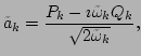
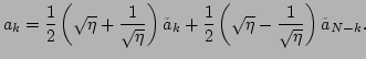
Consider the generalization of the transformation (2), namely, the transformation from the Fourier variables $Q_k$ and $P_k$ to the renormalized variables $\tilde{a}_k$ by

$$\tilde{a}_k=\frac{P_k-\imath \tilde{\omega}_kQ_k}{\sqrt{2\tilde{\omega}_k}},$$ (19)

where $\tilde{\omega}_k$ is an arbitrary function with the only restrictions

$$\tilde{\omega}_k>0,~~\tilde{\omega}_k=\tilde{\omega}_{N-k}.$$ (20)

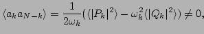
One can show that, these restrictions (20) provide a necessary and sufficient condition for the transformation (19) to be canonical. For the renormalized waves $\tilde{a}_k$, we can compute

$$\langle \tilde{a}_k^*\tilde{a}_l\rangle = \frac{1}{2\tilde{\omega}_k}(\langle \vert P_k\vert^2\rangle +\tilde{\omega}_k^2\langle \vert Q_k\vert^2\rangle )\delta^k_l,$$ (21)

$$\langle \tilde{a}_k\tilde{a}_l\rangle = \frac{1}{2\tilde{\omega}_k}(\langle \vert P_k\vert^2\rangle -\tilde{\omega}_k^2\langle \vert Q_k\vert^2\rangle )\delta^{k+l}_N.$$ (22)

Since we have the freedom of choosing any $\tilde{\omega}_k$ (with the only restrictions (20)), we can chose $\tilde{\omega}_k$ such that $\langle \tilde{a}_k\tilde{a}_{N-k}\rangle$ vanishes. Thus, the renormalized variables $\tilde{a}_k$ for a strongly nonlinear system will behave like the bare variables $a_k$ for a noninteracting system in terms of vanishing correlations between waves. Therefore, we determine $\tilde{\omega}_k$ via

$$\langle \vert P_k\vert^2\rangle -\tilde{\omega}_k^2\langle \vert Q_k\vert^2\rangle =0.$$ (23)

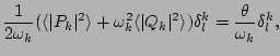
Note that the requirement (23) has the form of the virial theorem for the free waves but with the renormalized linear dispersion $\tilde{\omega}_k$. We rewrite Eq. (23) in terms of the kinetic and quadratic potential parts of the energy of the mode $k$ as

$$\frac{\tilde{\omega}_k}{\omega _k}=\sqrt{\frac{\langle K_k\rangle }{\langle U_k\rangle }}.$$ (24)

The in Eqs. (11) and (12) leads to the $k$ independence of the right-hand side of Eq. (24). This allows us to define the renormalization factor $\eta$ for all $k$'s by

$$\eta\equiv\frac{\tilde{\omega}_k}{\omega _k}=\sqrt{\frac{\langle K\rangle }{\langle U\rangle }}.$$ (25)

for dispersion $\omega _k$. Here $K=\sum_{k=1}^{N-1}K_k$ and $U=\sum_{k=1}^{N-1}U_k$ are the kinetic and the quadratic potential parts of the total energy of the system (9), respectively. Note that the way of constructing the renormalized variables $\tilde{a}_k$ via the precise requirement of vanishing correlations between waves yields the exact expression for the renormalization factor, which is valid for all wave numbers $k$ and any strength of nonlinearity. The independence of $\eta$ of the wave number $k$ is a consequence of the Gibbs measure. This $k$ independence phenomenon has been observed in previous numerical experiments [12,6]. We will elaborate on this point in the results of the numerical experiment presented in Section III.

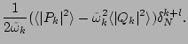
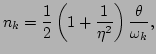
The immediate consequence of the fact that $\eta$ is independent of $k$ is that the power spectrum of the renormalized waves possesses the precise Rayleigh-Jeans distribution, i.e.,

$$\tilde{n}_k=\frac{\theta }{\tilde{\omega}_k},$$ (26)

from Eq. (21), where $\tilde{n}_k=\langle \vert\tilde{a}_k\vert^2\rangle$. Combining Eqs. (2) and (19), we find the relation between the ``bare'' waves $a_k$ and the renormalized waves $\tilde{a}_k$ to be

$$a_k=\frac{1}{2}\left(\sqrt{\eta}+\frac{1}{\sqrt{\eta}}\right)\tilde{a}_k+\frac{1}{2}\left(\sqrt{\eta}-\frac{1}{\sqrt{\eta}}\right)\tilde{a}_{N-k}.$$ (27)

Using Eq. (27), we obtain the following form of the power spectrum for the bare waves $a_k$

$$n_k=\frac{1}{2}\left(1+\frac{1}{\eta^2}\right)\frac{\theta }{\omega _k},$$ (28)

which is a modified Rayleigh-Jeans distribution due to the renormalization factor $(1+1/\eta^2)/2$. Naturally, if the nonlinearity becomes weak, we have $\eta\rightarrow 1$, and, therefore, all the variables and parameters with tildes reduce to the corresponding ``bare'' quantities, in particular, $\tilde{\omega}_k\rightarrow\omega _k$, $\tilde{a}_k\rightarrow a_k$, $\tilde{n}_k\rightarrow n_k$. It is interesting to point out that, even in a strongly nonlinear regime, the ``free-wave'' form of the Rayleigh-Jeans distribution is satisfied exactly [Eq. (26)] by the renormalized waves. Thus, we have demonstrated that even in the presence of strong nonlinearity, the system in thermal equilibrium can still be viewed statistically as a system of ``free'' waves in the sense of vanishing correlations between waves and the power spectrum.

Note that, in the derivation of the formula for the renormalization factor [Eq. (25)], we only assumed the nearest-neighbor interactions, i.e., the potential is the function of $q_j-q_{j+1}$. One of the well-known examples of such a system is the $\beta$-FPU chain, where only the forth order nonlinear term in $V$ is present. In the remainder of the article, we will focus on the $\beta$-FPU to illustrate the framework of the renormalized waves $\tilde{a}_k$.