Next: Linear theory without a
Up: text
Previous: Introduction
Linear dynamics of the GP equation
We will now develop a WKB theory for small-scale wave-packets,
described by a linearized GP equation, with and without the presence
of a background condensate. As is traditional with any WKB-type method
we assume the existence of a scale separation
 , as
explained in section
, as
explained in section ![[*]](file:/usr/share/latex2html/icons/crossref.png) . In this analysis we will take
. In this analysis we will take  so that any spatial derivatives of a given large-scale quantity
(e.g. the potential
so that any spatial derivatives of a given large-scale quantity
(e.g. the potential  or the condensate) are of order
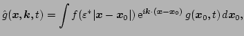
 . The transition to WKB phase-space is achieved through
the application of the Gabor transform [23],
. The transition to WKB phase-space is achieved through
the application of the Gabor transform [23],
 |
(2) |
where  is an arbitrary function fastly decaying at infinity.
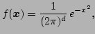
For our purposes it will be sufficient to consider a Gaussian of the form
where
is an arbitrary function fastly decaying at infinity.
For our purposes it will be sufficient to consider a Gaussian of the form
where  is the number of space dimensions. The parameter
 is small and such that
 . Hence, our kernel varies at the
intermediate-scale. A Gabor transform can therefore be thought of as a
localized Fourier transform, and in the limit
. Hence, our kernel varies at the
intermediate-scale. A Gabor transform can therefore be thought of as a
localized Fourier transform, and in the limit
 becomes an exact Fourier transform. Physically, one can view a Gabor
transform as a wavepacket distribution function over positions
becomes an exact Fourier transform. Physically, one can view a Gabor
transform as a wavepacket distribution function over positions
 and wavevectors
  .
.
Subsections
Next: Linear theory without a
Up: text
Previous: Introduction
Dr Yuri V Lvov
2007-01-23