Next: Equation for the multi-mode
Up: Evolution of statistics of
Previous: Evolution of statistics of
Let us consider the initial fields
 which are of the RPA type as defined above. We will perform
averaging over the statistics of the initial fields
in order to obtain an evolution equations, first for
which are of the RPA type as defined above. We will perform
averaging over the statistics of the initial fields
in order to obtain an evolution equations, first for  and
then for the multi-mode PDF.
Let us introduce a graphical classification of the above terms which
will allow us to simplify the statistical averaging and to understand
which terms are dominant. We will only consider here contributions from
and
then for the multi-mode PDF.
Let us introduce a graphical classification of the above terms which
will allow us to simplify the statistical averaging and to understand
which terms are dominant. We will only consider here contributions from
 and
and  which will allow us to understand the basic method.
Calculation of the rest of the terms,
which will allow us to understand the basic method.
Calculation of the rest of the terms,  ,
,  and
and  ,
follows the same principles and can be found in [24].
First,
The linear in
,
follows the same principles and can be found in [24].
First,
The linear in
 terms are represented by which, upon using
(34), becomes
terms are represented by which, upon using
(34), becomes
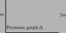
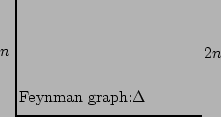
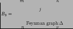
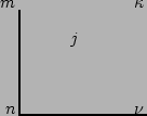
Let us introduce some graphical notations for a simple classification
of different contributions to this and to other (more lengthy)
formulae that will follow. Combination
 will
be marked by a vertex joining three lines with in-coming
will
be marked by a vertex joining three lines with in-coming  and
out-coming
and
out-coming  and
and  directions. Complex conjugate
 will be drawn by the same vertex but with the opposite
in-coming and out-coming directions. Presence of
will be drawn by the same vertex but with the opposite
in-coming and out-coming directions. Presence of  and
and  will be indicated by dashed lines pointing away and toward the vertex
respectively. 4 Thus, the two terms in formula (52)
can be schematically represented as follows,
will be indicated by dashed lines pointing away and toward the vertex
respectively. 4 Thus, the two terms in formula (52)
can be schematically represented as follows,
Let us average over all the independent phase factors in the set
 .
Such averaging takes into account the statistical
independence and uniform distribution of
variables
.
Such averaging takes into account the statistical
independence and uniform distribution of
variables  . In particular,
 ,
,
 and
and
 . Further, the products that involve
odd number of 's are always zero, and among the even
products only those can survive that have equal numbers of
's and
. Further, the products that involve
odd number of 's are always zero, and among the even
products only those can survive that have equal numbers of
's and  's. These 's and 's
must cancel each other which is possible if their indices
are matched in a pairwise way similarly to the Wick's
theorem. The difference with the standard Wick, however, is
that there exists possibility of not only internal
(with respect to the sum) matchings but also external
ones with 's in the pre-factor
's. These 's and 's
must cancel each other which is possible if their indices
are matched in a pairwise way similarly to the Wick's
theorem. The difference with the standard Wick, however, is
that there exists possibility of not only internal
(with respect to the sum) matchings but also external
ones with 's in the pre-factor
 .
.
Obviously, non-zero contributions can only arise for terms in which
all 's cancel out either via internal mutual couplings within
the sum or via their external couplings to the 's in the
 -product. The internal couplings will indicate by joining the
dashed lines into loops whereas the external matching will be shown as
a dashed line pinned by a blob at the end. The number of blobs in
a particular graph will be called the valence of this graph.
-product. The internal couplings will indicate by joining the
dashed lines into loops whereas the external matching will be shown as
a dashed line pinned by a blob at the end. The number of blobs in
a particular graph will be called the valence of this graph.
Note that there will be no
contribution from the internal couplings between the incoming and the
out-coming lines of the same vertex because, due to the
 -symbol, one of the wavenumbers is 0 in this case, which means
5that
-symbol, one of the wavenumbers is 0 in this case, which means
5that  . For we have
with
and
which correspond to the following expressions,
and
Because of the -symbols involving  's, it takes very
special combinations of the arguments in
's, it takes very
special combinations of the arguments in
 for the
terms in the above expressions to be non-zero. For example, a
particular term in the first sum of (53) may be non-zero if
two 's in the set
for the
terms in the above expressions to be non-zero. For example, a
particular term in the first sum of (53) may be non-zero if
two 's in the set
 are equal to 1 whereas the rest of
them are 0. But in this case there is only one other term in this sum
(corresponding to the exchange of values of and ) that may be
non-zero too. In fact, only utmost two terms in the both
(53) and (54) can be non-zero simultaneously. In
the other words, each external pinning of the dashed line removes
summation in one index and, since all the indices are pinned in the
above diagrams, we are left with no summation at all in i.e. the
number of terms in is
are equal to 1 whereas the rest of
them are 0. But in this case there is only one other term in this sum
(corresponding to the exchange of values of and ) that may be
non-zero too. In fact, only utmost two terms in the both
(53) and (54) can be non-zero simultaneously. In
the other words, each external pinning of the dashed line removes
summation in one index and, since all the indices are pinned in the
above diagrams, we are left with no summation at all in i.e. the
number of terms in is  with respect to large
  . We will
see later that the dominant contributions have
. We will
see later that the dominant contributions have  terms. Although these terms come in the
 order, they will be
much greater that the
order, they will be
much greater that the
 terms because the limit
 must always be taken before
 .
.
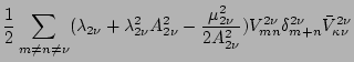
Let us consider the first of the
-terms, . Substituting
(34) into (48), we have
where
Here the graphical notation for the interaction coefficients  and
the amplitude
and
the amplitude  is the same as introduced in the previous section and
the dotted line with index indicates that there is a summation over
but there is no amplitude in the corresponding expression.
is the same as introduced in the previous section and
the dotted line with index indicates that there is a summation over
but there is no amplitude in the corresponding expression.
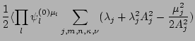
Let us now perform the phase averaging which corresponds to the internal and external
couplings of the dashed lines. For
 we have
 |
|
|
(51) |
where
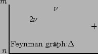
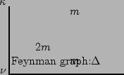
We have not written out the third term in (57) because
it is just a complex conjugate of the second one. Observe that all the
diagrams in the first line of (57) are with
respect to large because all of the summations are lost due to the
external couplings(compare with the previous section). On the other
hand, the diagram in the second line contains two purely-internal
couplings and is therefore . This is because the number of
indices over which the summation survives is equal to the number of
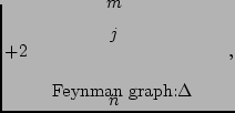
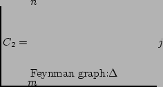
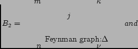
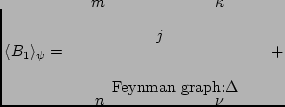
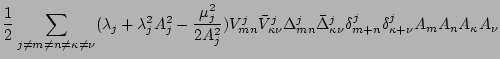
purely internal couplings. Thus, the zero-valent graphs
are dominant and we can write
![$\displaystyle \langle B_1\rangle_\psi = \prod_l\delta(\mu_l)\sum_{j,m,n}(\lambd...
...}^{j}\vert^2
\vert\Delta_{mn}^{j}\vert^2
\delta_{m+n}^{j}A_m^2A_n^2[1+O(1/N^2)]$](img305.png) |
|
|
(52) |
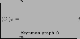
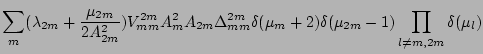
Now we are prepared to understand a general rule: the dominant contribution
always comes from the graphs with minimal valence, because each external
pinning reduces the number of summations by one. The minimal valence of
the graphs in
 is one and, therefore,
is order times smaller than
is one and, therefore,
is order times smaller than
 .
On the other hand,
.
On the other hand,
 is of the same order as
, because it contains zero-valence graphs. We have
is of the same order as
, because it contains zero-valence graphs. We have
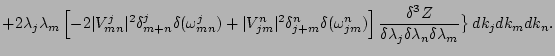
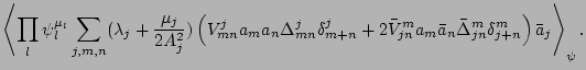
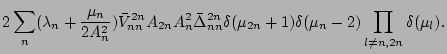
Summarising, we have
![$\displaystyle J_2 = \prod_{l}\delta(\mu_l)\sum_{j,m,n}(\lambda_{j}+\lambda_{j}^...
... \vert\Delta_{jn}^{m}\vert^2 \delta_{j+n}^{m}
\right]
A_m^2A_n^2 \; [1+O(1/N)].$](img312.png) |
|
|
(54) |
Thus, we considered in detail the different terms involved
in and we found that the dominant contributions come
from the zero-valent graphs because they have more summation
indices involved. This turns out to be the general rule in both three-wave and
four-wave cases and it
allows one to simplify calculation by discarding a significant
number of graphs with non-zero valence.
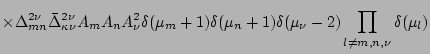
Calculation of terms
to can be found in [24] and here we only present the
result,
![$\displaystyle J_3 = 4 \prod_l\delta(\mu_l) \sum_{j,m,n} \lambda_j \left[ - \ver...
...0,-\omega_{jn}^m)\delta_{j+n}^m (A_m^2 -A_n^2) \right] A_j^2 \times [1+O(1/N)],$](img313.png) |
(55) |
 (i.e. is order
  times smaller than or ) and
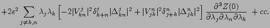
![$\displaystyle J_5= 2 \prod_l\delta(\mu_l) \sum_{j\neq k,n}\lambda_j\lambda_k \l...
...ta_{j+k}^n \vert\Delta_{jk}^n\vert^2 \right] A_j^2 A_n^2 A_k^2 \;\; [1+O(1/N)].$](img316.png) |
(56) |
Using our results for  in (46) and (45) we have
Here partial derivatives with respect to  appeared because of
the
appeared because of
the  factors.
This expression is valid up to
factors.
This expression is valid up to
 and
and
 corrections.
Note that we still have not used any assumption about the statistics
of
corrections.
Note that we still have not used any assumption about the statistics
of  's.
Let us now
limit followed by
's.
Let us now
limit followed by
 (we re-iterate that this order of the limits is essential).
Taking into account that
(we re-iterate that this order of the limits is essential).
Taking into account that
 , and
, and
 and,
replacing
and,
replacing
 by
by  we have
Here variational derivatives appeared instead of partial derivatives because of
the
limit.
Now we can observe that the
evolution equation for does not involve which
means that if initial
contains factor
 it will be preserved at all time.
This, in turn, means that the phase factors remain a set of statistically independent (of each each other and
of 's) variables uniformly distributed on
it will be preserved at all time.
This, in turn, means that the phase factors remain a set of statistically independent (of each each other and
of 's) variables uniformly distributed on  . This is true with
accuracy
. This is true with
accuracy
 (assuming that the -limit is taken first, i.e.
 ) and this proves persistence of the first of the
``essential RPA'' properties. Similar result
for a special class of three-wave systems arising in the solid state physics
was previously obtained by Brout and Prigogine [20].
This result is interesting
because it has been obtained without any assumptions on the
statistics of the amplitudes
) and this proves persistence of the first of the
``essential RPA'' properties. Similar result
for a special class of three-wave systems arising in the solid state physics
was previously obtained by Brout and Prigogine [20].
This result is interesting
because it has been obtained without any assumptions on the
statistics of the amplitudes  and, therefore, it is valid
beyond the RPA approach. It may appear useful in future for study of
fields with random phases but correlated amplitudes.
and, therefore, it is valid
beyond the RPA approach. It may appear useful in future for study of
fields with random phases but correlated amplitudes.
Next: Equation for the multi-mode
Up: Evolution of statistics of
Previous: Evolution of statistics of
Dr Yuri V Lvov
2007-01-23


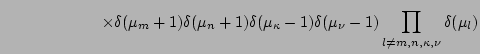


![$\displaystyle \parbox{25mm} {
\begin{fmffile}{n19p}
\begin{fmfgraph*}(70,50) \f...
...s_arrow, left=.7, label= $n$}{v2,v1}
\end{fmfgraph*}\end{fmffile}}
[1+O(1/N^2)]$](img310.png)
![$\displaystyle %YL
=2 \prod_{l}\delta(\mu_l)\sum_{j,m,n}(\lambda_{j}+\lambda_{j}...
...vert^2 \vert\Delta_{jn}^{m}\vert^2 \delta_{j+n}^{m}A_m^2A_n^2 \; [1+O(1/N^2)]
,$](img311.png)
![$\displaystyle {\epsilon}^2
\sum_{j,m,n}(\lambda_{j}+\lambda_{j}^2 {\partial \ov...
...n}^{m}
\right]
{\partial^2 Z(0)\over \partial \lambda_{m} \partial \lambda_{n}}$](img319.png)
![$\displaystyle + 4{\epsilon}^2 \sum_{j,m,n}
\lambda_j
\left[ - \vert V_{mn}^j\ve...
...partial \lambda_{n}} \right)
\right]
{\partial Z(0) \over \partial \lambda_{j}}$](img320.png)
![$\displaystyle 4 \pi {\epsilon}^2
\int \big\{ (\lambda_{j}+\lambda_{j}^2 {\delta...
...delta_{j+n}^{m}
\right]
{\delta^2 Z\over \delta \lambda_{m} \delta \lambda_{n}}$](img331.png)
![$\displaystyle + 2
\lambda_j
\left[ - \vert V_{mn}^j\vert^2 \delta(\omega_{mn}^j...
...a \over \delta \lambda_{n}} \right)
\right]
{\delta Z \over \delta \lambda_{j}}$](img332.png)