Conservation Laws, Thermodynamic and Finite-Flux solutions of the Kinetic Equation.

The collision integral in (2.20) has the following constants of motion

$${\cal N}= \frac{V}{(2\pi)^d} \int d {\bf k} n_k, {\cal ... ...i)^d} \int \frac{\hbar^2\vert\vec k\vert^2}{2m} d {\bf k} n_k,$$ (3.1)

which can be identified as number of particles, momentum and kinetic energy. In a spatially homogeneous systems, ${\bf P}=0$ so that the only relevant constants of motion are $\cal N$ and $\cal E$.

In this article we will be dealing with the isotropic case only, and, for simplicity, neglect the spin degree of freedom. Therefore we simplify the collision integral by averaging it over all angles. First, we change variables from particles momentum $\bf k$ to the particle kinetic energy

$$\epsilon _k=\hbar \omega _k=\frac{\hbar^2 k^2}{2 m},$$ (3.2)

where $m$ is the coefficient of proportionality between $\omega _k$ and $\hbar k^2/2$, and can be associated with (effective) mass of the interacting particles.

We introduce $n_{\omega }=n({\bf k}(\omega ))$ and rewrite the kinetic equation as

$$\dot n_\omega = \frac{1}{\Omega _0 k^{d-1} (dk/d\omega )}\times \int\int\limits_{\omega _i>0,i=1,2,3}\int{\cal K}(\omega ,\omega _1,\omega _2,\omega _3) S_{\omega \omega _1 \omega _2 \omega _3}$$

$$\times\delta (\omega +\omega _1-\omega _2-\omega _3) d\omega _1d\omega _2d\omega _3$$

where $S_{\omega \omega _1 \omega _2 \omega _3}$ is the angle-averaged potential,

$$S_{\omega \omega _1 \omega _2 \omega _3}=4\pi\Omega _0(k k_1 ... ..._2k_3}\vert^2 \delta ({\bf k}+{\bf k_1}-{\bf k_2}-{\bf k_3})>.$$ (3.3)

The brackets $<..>$ denote averages over unit spheres (including the $\frac{V}{(2\pi)^d}$ factors) in ${\bf k},{\bf k_1},{\bf k_2},{\bf k_3}$ space (i.e., we have integrated over all angular contributions) and $\Omega _0$ is the surface area of the unit sphere in $d$ dimensions. Although in our case $d=3$, we want to stress with the above notation the results can easily be extended to other dimensions, for example to $d=2$ which is appropriate for the description of semiconductor quantum wells. $\cal K$ is the kernel of kinetic equation, which for the quantum (fermionic), quantum (bosonic) and classical cases is given respectively by:

$${\cal K^{\rm fermionic}}(\omega ,\omega _1,\omega _2,\omega _3) = n_{\omega _2} n_{\omega _3} (1-n_{\omega _1})(1-n_{\omega }) - n_{\omega } n_{\omega _1} (1-n_{\omega _2})(1-n_{\omega _3}),$$

$${\cal K}^{\rm bosonic} (\omega ,\omega _1,\omega _2,\omega _3) = (n_{\omega _2} n_{\omega _3}(n_{\omega }+n_{\omega _1}+1)-n_{\omega } n_{\omega _1} (n_{\omega _2}+n_{\omega _3}+1)),$$

$${\cal K^{\rm classical}}({\omega ,\omega _1,\omega _2,\omega _3}) = (n_{\omega _2} n_{\omega _3}(n_{\omega }+n_{\omega _1})-n_{\omega } n_{\omega _1} (n_{\omega _2}+n_{\omega _3})).$$ (3.4)

We then introduce the particle density per frequency

$$N_\omega ={\Omega _0 k^{d-1} (dk/d\omega )}n_\omega$$

so that $\int N_\omega d\omega =\int n_k d{\bf k}$ and

$$\dot N_\omega = \int\limits_{\omega _1,\omega _2,\omega _3>0}\int... ...}\delta (\omega +\omega _1-\omega _2-\omega _3) d\omega _1d\omega _2d\omega _3.$$

One class of steady (equilibrium) solutions of the KE corresponds to the thermal equilibrium. For fermionic systems, it is given by the Fermi Dirac (FD) distribution, and for bosonic systems it is given by the Bose-Einstein distribution,

$$n_{k}=\frac{1}{\exp{(\beta (\epsilon _k-\mu))}\pm 1}$$ (3.5)

where the plus sign corresponds to the fermion case and the minus sign to the bosonic case. $\mu$ is the chemical potential and $\beta$ is the inverse temperature in energy units. The classical analogue of the quantum thermal equilibrium distribution is given by the Rayleigh-Jeans distribution

$$n(k)=T/(\mu + \epsilon _k) .$$ (3.6)

It is easy to check that the solutions (3.7,3.8) make the integrand in (3.3,3.6) exactly zero in all three cases.

However, the thermodynamic equilibrium is not the most general steady (equilibrium) solution of the kinetic equation and indeed in some cases has little relevance. The solutions we are most interested in are those which describe the steady state reached between ranges of frequencies where particles and energy are added to or removed from the system. These regions, where there is no pumping or dumping, are called "windows of transparency" or "inertial ranges". In particular, we have in mind the following situation. Particles and energy are added to the system in a narrow range of intermediate frequencies about $\omega _0$. Particles and energy are drained from the system in a range of frequencies about $\omega <\omega _L<\omega _0$ and for $\omega >\omega _R>\omega _0$. Because of conservation of energy and particles in the inertial ranges between $\omega _L$ and $\omega _0$ and between $\omega _0$ and $\omega _R$ where there is no pumping or damping and because the relations between particle number $N_\omega$ and energy density $E_\omega =\omega N_\omega$, we will find that a net flux of energy to the higher frequencies must be accompanied by a net flux of particles to lower frequencies as it might be expected by analogy with classical wave turbulence. The presence of sources and sinks drives the system away from the thermodynamic equilibrium. Therefore, in the windows of transparency, $\omega _L<\omega <\omega _0$ and $\omega _0<\omega <\omega _R$, the system can also relax to equilibrium distributions corresponding to a finite flux of particles and energy flowing through these windows from the sources to the sinks. These are the new solutions of the QKE. The number of such finite flux solutions corresponds to the number of conserved densities (here two, $n_k$ and $\omega _k n_k$, or $N_\omega$ and $\omega N_\omega$) of the QKE.

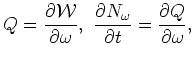
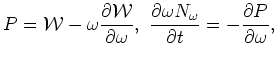
To demonstrate the existence of such solutions, we rewrite the KE in the following form:

$$\dot N_\omega = \frac{\partial^2}{\partial \omega ^2} {\cal W}[n_\omega ],$$

$${\cal W}[n_\omega ] = \int\int\limits_\Omega \int (\omega +\omega _1-\omega _2-\omega _... ...ega _2+\omega _3-\omega ,\omega _2,\omega _3} d\omega _1 d\omega _2 d\omega _3,$$

where the integration is over the region $\Omega \{\omega _1,\omega _2,\omega _3>0 \omega _1<\omega _2+\omega _3<\omega +\omega _1\}$ This expression can be checked by direct differentiation.

The relevant equation kinetic equation, which includes the presence of sources and sinks is

$$\frac{\partial N_\omega }{\partial t}= \frac{\partial^2}{\partial\omega ^2}{\cal W}[n_\omega ]+F_\omega -D_\omega ,$$ (3.7)

where we think of $F_\omega$ as having its support near $\omega =\omega _0$ and $D_\omega$ its support below $\omega _L$ and above $\omega _R$. We ask if (3.10) leads to a steady (equilibrium) solutions in the transparency regions $\omega _L<\omega <\omega _0$ and $\omega _0<\omega <\omega _R$ where $F_\omega =D_\omega =0$ corresponding to a finite flux of particles and energy across these windows. One can readily associate the quantities

$$Q=\frac{\partial {\cal W}}{\partial \omega }, \frac{\partial N_\omega }{\partial t}=\frac{\partial Q}{\partial \omega },$$

$${\rm and } \$$

$$P={\cal W} -\omega \frac{\partial {\cal W}}{\partial \omega }, \frac{\partial \omega N_\omega }{\partial t}=-\frac{\partial P}{\partial \omega },$$ (3.8)

with the fluxes $P$ and $Q$ of particles $N_\omega$ and energy $E_\omega =\omega N_\omega$. $Q$ and $P$ are taken positive if leftward and rightward flowing respectively. In the windows of transparency, we look for solutions for which $N_\omega$ is constant in time and then (3.9) integrates to

$${\cal W}=Q\omega +P$$ (3.9)

where $Q$ and $P$ are constants. The two parameter family of thermodynamic solutions, parametrized by $T$ and $\mu$ is given by solving the homogeneous equation ${\cal W}=0$ for which $P=Q=0$. Therefore, the thermodynamic solutions carry no fluxes of particles or energy. A more general³ steady (equilibrium) solution to (3.9) therefore is the four-parameter family

$$n_\omega =n_\omega (T,\mu,P,Q).$$ (3.10)

We are particularly interested in the solutions for which $Q_0$ particles per unit time and $\omega _0 Q_0$ units of energy per unit time are fed to the system in a narrow frequency window about $\omega =\omega _0$. We will assume that the flux of particles passing through the left (right) window $\omega _L<\omega <\omega _0$ ( $\omega _0<\omega <\omega _R$) is $Q_L$ ($Q_R$) and the flux of energy though the right (left) window is $P_R$ ($P_L$). We will also assume that the sinks consume all the particles and energy that reach them. Then (see Figure 1)

$$Q_L-Q_R=Q_0$$

$$P_R-P_L=\omega _0 Q_0$$

$$P_L=-\omega _L Q_L$$

$$Q_R=-\frac{1}{\omega _R} P_R.$$ (3.11)

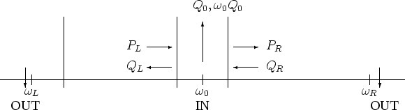
Figure 1

The first two relations in (3.14) express conservation of particles and energy. The second two express the fact that, in order to maintain equilibrium, the rate of particle destruction at $\omega _R$ is the rate of energy destroyed there divided by the energy per particle. Likewise the amount of energy destroyed at $\omega _L$ (which absorption, in the context of application discussed in the section 5, will be due to semiconductor lasing) must be $\omega _L$ times the number of particles absorbed there. Solving (3.14) we obtain

$$Q_L = Q_0 (\omega _R-\omega _0)/(\omega _R-\omega _L),$$

$$Q_R = -Q_0(\omega _0-\omega _L)/(\omega _R-\omega _L),$$

$$P_R = Q_0 \omega _R (\omega _0-\omega _L)/(\omega _R-\omega _L)$$

$$P_L = -\omega _L Q_0 (\omega _R-\omega _0)/(\omega _R-\omega _L).$$ (3.12)

We see that for $\omega _L\ll\omega _0\ll\omega _R$, $\vert Q_R\vert\ll Q_L\simeq Q_0, \vert P_L\vert\ll P_R\simeq \omega _0 Q_0$ so that the solutions are almost pure Kolmogorov in the sense that almost all energy flows to $\omega _R$ and almost all particles flow to $\omega _L$. However, it is important to stress that in the left window, (3.12) becomes

$${\cal W}=Q_L(\omega -\omega _L)$$ (3.13)

and in the right window

$${\cal W}=P_R(1-\frac{\omega }{\omega _R})$$ (3.14)

so that the right hand sides vanish if the frequency approaches the sink value. This aids convergence in these windows.

Solutions to (3.16), (3.17) have not been investigated even in the classical case. In the classical case, Zakharov (see, e.g., [22],[23]) had found the pure Kolmogorov solutions $T=\mu=P=0$, $T=\mu=Q=0$ which turns out to have power law behavior $n_{\omega }=c\omega ^{-x}$. Likewise, in the bosonic case, several authors have attempted to find power law solutions which essentially balance the quadratic terms in ${\cal W}^{\rm bosonic}$ with a finite energy flux. However, in the differential approximation, there are no power law solutions.

In many cases it may be that whenever $\omega _R\gg\omega _0$, $\omega _L$ may not be all that much smaller than $\omega _0$. In particular, in order to exploit these solutions in the context of semiconductor lasers, it is advantageous to have $\omega _0$ close enough to $\omega _L$ to minimize energy losses (the ratio $P_R/\vert P_L\vert=\omega _R(\omega _0-\omega _L)/( \omega _L(\omega _R-\omega _0))$) but far enough away to facilitate pumping unimpeded by Pauli blocking. We return to this application after introducing an enormous simplification for $\cal W$ which gives a very good qualitative description of the collision integral.